


Gradient Boosting Machines 是一個超級受歡迎的機器學習法,在許多領域上都有非常成功的表現,也是Kaggle競賽時常勝出的主要演算法之一。有別於隨機森林集成眾多深且獨立的樹模型,GBM則是集成諸多淺且弱連續的樹模型,每個樹模型會以之前的樹模型為基礎去學習和精進,結果通常是難以擊敗的。
套件與資料準備
|
1 2 3 4 5 6 7 8 9 |
library(rsample) # data splitting library(gbm) # basic implementation library(xgboost) # a faster implementation of gbm library(caret) # an aggregator package for performing many machine learning models library(h2o) # a java-based platform library(pdp) # model visualization library(ggplot2) # model visualization library(lime) # model visualization library(vtreat) |
使用AmesHousing套件中的Ames Housing數據,並將數據切分為7:3的訓練測試比例。
|
1 2 3 4 5 6 |
# Create training (70%) and test (30%) sets for the AmesHousing::make_ames() data. # Use set.seed for reproducibility set.seed(123) ames_split ames_train ames_test |
tree-based演算法往往可以將未處理資料配適的很好(即不需要特別將資料進行normalize, center,scale),所以在以下筆記中將聚焦在如何使用多種不同套件執行GBMs。而雖然在這邊沒有去進行資料前處理,但我們仍可花時間透過處理變數特徵使得模型成效更佳。
Gradient Boosting Machines’ Advantage & Disadvantages
優勢
- 產生的預測精準度通常無人能打敗
- 擁有許多彈性 – 可以針對不同的Loss Function來進行優化(*Loss Function即所有需要被「最小化」的目標函式,一個最常用來尋找使目標函式最小值的資料點的方法即為gradient descent),且有hyperparameters的參數選項可以tuning,好讓目標函式配適的很好。
- 不需要資料前處理 – 通常可以很好的處理類別和數值型變數。
- 可以處理遺失值 – 不需要空值填補。
劣勢
- GBMs會持續優化模型來最小化誤差。這樣可能會過度擬和極端值的部分而造成過度配適。因此必須綜合使用cross validation來銷除這個情況。
- 計算上成本非常高 – GBMs通常會包含許多樹(>1000),會佔用許多時間和記憶體。
- 模型彈性度高,導致許多參數會影響grid search的流程(比如說迭代次數,樹的深度,參數正規化等等),在tuning模型的時候會需要大型的grid search過程。
- 可解釋程度稍稍少了一點,但有許多輔助工具如變數重要性、partial dependence plots, LIME等。
Gradient Boosting Machines (GBMs) 概念
許多監督式機器學習模型都是建立在單一預測模的基礎上(比如說linear regression, penalized models or regularized regression, naive Bayes, support vector machines)。而則有像是Bagging和Random Forests這種集成學習演算法(ensemble learning),集成眾多預測模型並單純平均每個模型的預測結果得出預測值。另外一種則是Boosting系列,是基於不一樣的建設性策略來進行集成學習。
Boosting的主要概念就是將新模型「有順序、循序漸進」的加入集成學習。在每一次迭代中,會新增一個新的(new)、弱的(weak)、base-learner模型,針對到目前為止集成學習的誤差進行訓練。
以下進一步解釋boosting models的特徵關鍵字:
- Base-learning models: Boosting是一個迭代改善任何弱學習模型的框架。許多Gradienet Boosting應用可允使用者任意加入眾多類型的weak learners模型。然而在實務上,boosted algorithm幾乎總是使用Decision Trees當作base-learner。也因此本學習筆記會主要討論boosting regression trees的應用。
- Training weak models: 所謂的「弱模型(weak model)」指的是模型的錯誤率只有稍稍比隨機猜測好一點點的模型。Boosting背後的概念就是每一個順序模型都會建立一個僅稍稍改善殘餘誤差的弱模型(weak model)。以決策樹來說,較淺的樹就是弱模型的代表。一般來說,淺的決策樹模型切割數約在1~6之間。綜合多個弱模型會有以下好處(將較於綜合多個強模型):
- 速率: 建構弱模型在計算成本上是便宜的。
- 精準度的改善: weak model允許演算法「慢慢學習」;即在模型表現不好的新領域進行些微調整。一般來說,慢慢學習的統計方法通常表現不錯。
- 避免overfitting: 由於在集成學習過程中,每一次訓練模型僅稍稍貢獻一點點額外的成效改善,使得我們有辦法即時在偵測到overfitting時即停止學習(使用的cross validation)。
- 針對集成學習的殘餘誤差有順序性的訓練: Boosted trees是有順序性的;每一個樹模型都是依據前面的樹模型所得的資訊而訓練而成。基本的boosted regression trees演算法可被一般化為以下步驟(其中x代表features而y代表目標回應變數):
- 依據原始資料配適一棵樹模型: \(F_{1}(x) = y\)
- 並依據先前的殘餘誤差訓練下一棵樹模型: \(h_{1}(x) = y – F_{1}(x)\)
- 將新的樹新增到演算法:\(F_{2}(x) = F_{1}(x) + h_{1}(x)\)
- 再一次依據殘餘誤差訓練下一棵樹模型 = \(h_{2}(x) = y – F_{2}(x)\)
- 將新的樹新增到演算法:\(F_{3}(x) = F_{2}(x) + h_{2}(x)\)
- 持續這個過程直到一些機制(如cross validation)告訴演算法可以停止。
boosted regression trees的基本演算法概念可以一般化為以下,即最終模型是b個獨立的回歸樹模型階段性相加的結果:
\[ f(x) = \sum_{b=1}^B f^b(x) \]
Gradient descent
許多演算法,包括Decision trees,都聚焦在最小化殘差,也因此皆強調「MSE Loss Function」的目標函式。上面所討論到的演算法摘要了boosting法如何循序漸進地利用有順序新的弱回歸樹模型來配飾真實資料趨勢並最小化誤差。這個就是gradient boosting用來最小化Meas Squared Error (MSE) Loss Funciton的方法。雖然有時候我們會想要聚焦在其他Loss function上,如Mean Absolute Error(MAE),或是遇到分類問題時所使用的deviance。而gradient boosting machines的命名則是取自於這個方法可以擴張至除了MSE以外的Loss function。
Gradient Boosting被認為是一個gradient descent(梯度下降)的演算法。Gradient Descent是一個非常通用的最適化演算法,能夠找到解決各種問題的最佳解。Gradient Descent的概念就是迭代的微調整參數來來最小化損失函數Loss Funciton。Gradient Descent會在給定的一組參數\(\theta\)區間,衡量局部Loss(cost) function的gradient,並沿著gradient下降的方向。直到gradient為0時,則找到局部最小值。
Gradient descent可以被應用在任意可微分的loss function上,所以讓GBMs可以針對感興趣的loss function來尋找最適解。在gradient descent中一個重要的參數就是由_learning rate_s所決定的每次的變動率(size of steps)。較小的變動率會使得模型訓練過程中會迭代多次來尋找最小值,而過高的變動率則可能會讓模型錯過最小值和遠遠偏離初始值。
此外,並不是所有的loss function都是凸形的(convex)(如碗型)。可能會有局部的最小值、平坦高原或不規則地形等,使得尋找global minimum變得困難。Stochastic gradient descent(隨機梯度下降)則可處理這樣的問題,透過抽樣一部分比例的觀察值(通常不重複),並使用此子集合建立下一個模型。這使得演算法變得更快一些,但是隨機抽樣的隨機性亦造成下降的loss function gradient的隨機性。雖然這個隨機性使得演算法無法找到absolute global minimum(全域最小值),但隨機性確實能讓演算法跳脫local minimum(局部最小值)、平坦高原等局部解,並接近全域的最小值。
我們在下一個階段即能看到如何透過多種hyperparameters參數選項來調整如何處理loss function的gradient descent。
Tuning
GBMs的好處與壞處就是該演算法提供多個調整參數。好處是GBMs在執行上非常具彈性,但壞處就是在調整與尋找最適參數組合上會很耗時。以下為幾個GBMs最常見的調整hyperparameters參數:
- 決策樹模型的數量:總共要配適的決策樹模型數量。GBMs通常會需要很多很多樹,但不像random Forests,GBMs是可以過度擬和(overfit)的,所以他演算的目標是尋找最適決策樹數量使得感興趣的loss function最小化。
- 決策樹的深度:d,每棵樹模型的切割(split)數。用來控制boosted集成模型的複雜度。通常\(d=1\)的效果不錯,即此弱模型是由一次分割所得的樹模型所組成。而更常見的split數可能介在\(1
- Learning rate: 決定演算法計算gradient descent的速率。較慢的learning rate速率,可以避免overfitting的機會,但同時也會增加尋找最適解的時間。learning rate也被稱作shrinkage。
- subsampling: 控制是否要使用原始訓練資料部分比例的抽樣子集合。使用少於100%的訓練資料表示你將使用stochastic gradient descent,這將有助於避免overfitting以及陷在loss function gradient的局部最小最大值。
而在本學習筆記中,亦會介紹到專屬於特定package的調整hyperparameters參數,用來改善模型成效以及模型訓練與調整的效率。
使用R實作Gradient Boosting Machines
有很多執行GBMs和GBM變種的套件。而本學習筆記會cover到的幾個最受歡迎的套件,包括:
- gbm: 最原始的執行GBMs的套件。
- xgboost: 一個更快速且有效的gradient boosting架構(後端為c++)。
- h2o: 強大的java-based的介面,提供平行分散演算法和高銷率的生產。
gbm
gbm套件是R裡面最原始執行GBM的套件。是來自於Freund & Schapire’s AdaBoost algorithm的Friedman’s gradient boosting machine延伸。由Mark Landry撰寫的GBM套件簡報可參考此連結。
gbm套件幾個功能與特色包括:
- Stochastic GBM(隨機 GBM)
- 可支援到1024個factor levels
- 支援「分類」和「回歸」樹
- 包括許多loss functions
- 提供Out-of-bag 估計法來尋找最適的迭代次數
- 容易overfitting – 因為套件中沒有自動使用提早煞車功能來偵測overfitting
- 如果內部使用cross-validation,這可以被平行分散到所有機器核心
- 目前gbm套件正在進行重新建構與重寫(並已持續一段時間)。
基本的gbm實作
gbm套件中有兩個主要的訓練用函數:gbm::gbm跟gbm::fit。
- gbm::gbm – 使用「formula介面」來設定模型。
- gbm::fit – 使用「x & y矩陣」來設定模型。
當變數量很大的時候,使用「x & y 矩陣」會比「formula」介面來的更有效率。
gbm()函數預設的幾個參數值如下:
- learning rate(shrinkage):0.1。學習步伐,通常越小的學習步伐會需要越多模型數(n.tree)來找到最小的MSE。而預設n.tree為100,是相當足夠的。
- number of trees(n.tree): 100。總迭代次數(新增模型數)。
- depth of tree(interaction.depth): 1。最淺的樹(最弱的模型)。
- bag.fraction: 0.5。訓練資料集有多少比例會被抽樣做為下一個樹模型的基礎。用來替模型注入隨機性。
- train.fraction: 1。模型首次使用訓練資料的比例,剩餘的觀測資料則最為OOB sample用來估計loss function用。
- cv.folds: 0。如果使用>1的cross validation folds,除了會回傳該參數組合下的模型配適結果,也會估計cv.error。
- verbose: 預設為FALSE。決定是否要印出程序和成效指標。
- n.cores: 使用的CPU核心數。由於在使用cross validation的時候,loop會將不同CV folds分配到不同核心。沒特別設定的話會使用偵測機器核心數函數來處理parallele::detectCores。
以下我們來建立一個學習步伐為0.001且模型數量為10000的GBMs。並使用5 folds的交叉驗證計算cross-validated error。
|
1 2 3 4 5 6 7 8 9 10 11 12 13 14 15 16 17 |
# 使抽樣結果可以重複 set.seed(123) # train GBM model system.time( gbm.fit formula = Sale_Price ~ ., distribution = "gaussian", data = ames_train, n.trees = 10000, # 總迭代次數 interaction.depth = 1, # 弱模型的切割數 shrinkage = 0.001, # 學習步伐 cv.folds = 5, # cross validation folds n.cores = NULL, # will use all cores by default verbose = FALSE ) ) |
|
1 2 3 |
## user system elapsed ## 23.348 0.332 80.086 |
GBMs模型約花80秒(約1分多鐘)。
將模型結果印出。結果包括文字資訊以及每一次迭代次數所對應的loss function(squared error loss)變化。
|
1 |
print(gbm.fit) |
|
1 2 3 4 5 6 7 8 |
## gbm(formula = Sale_Price ~ ., distribution = "gaussian", data = ames_train, ## n.trees = 10000, interaction.depth = 1, shrinkage = 0.001, ## cv.folds = 5, verbose = FALSE, n.cores = NULL) ## A gradient boosted model with gaussian loss function. ## 10000 iterations were performed. ## The best cross-validation iteration was 10000. ## There were 80 predictors of which 45 had non-zero influence. |
模型結果資訊是由list所儲存。可以使用索引的方式取出。
比如說我們來看最小的CV RMSE值。
|
1 |
sqrt(min(gbm.fit$cv.error)) |
|
1 2 |
## [1] 29133.33 |
表示平均來說模型估計值離真實Sale_Price差了約30K。
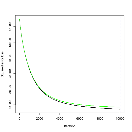
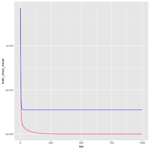
我們也可以透過以下方式將GBMs找尋最佳迭代數的過程繪出:(其中黑線的為訓練誤差(train.error),綠線為cv.error, 若method使用“test”,則會有紅線表示valid.error)
|
1 |
gbm.perf(object = gbm.fit, plot.it = TRUE,method = "cv") |
|
1 2 |
## [1] 10000 |
可以發現以此小學習步伐(0.001),會需要很多模型來接近最小的loss function(使cv.error最小化),最佳迭代數為10000。
Tuning
「手動tuning」
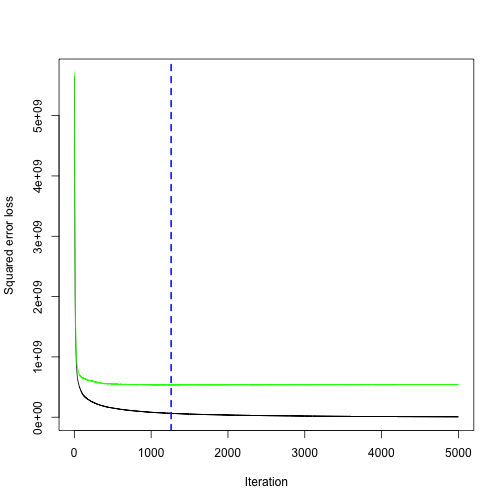
假設我們將學習步伐加大為0.1,迭代模型數降低為5000,且模型複雜度增加到3 splits。
|
1 2 3 4 5 6 7 8 9 10 11 12 13 14 15 16 17 |
# for reproducibility set.seed(123) # train GBM model system.time( gbm.fit2 formula = Sale_Price ~ ., distribution = "gaussian", data = ames_train, n.trees = 5000, interaction.depth = 3, shrinkage = 0.1, cv.folds = 5, n.cores = NULL, # will use all cores by default verbose = FALSE ) ) |
|
1 2 3 |
## user system elapsed ## 35.555 1.314 151.695 |
調大步伐後(0.1),花的時間變多為151秒(2.5分鐘),GBMs模型最小cv.error變得更低(23K)。
(v.s.小步伐(0.001)的cv.error: 29K)
|
1 |
sqrt(min(gbm.fit2$cv.error)) |
|
1 2 |
## [1] 23112.1 |
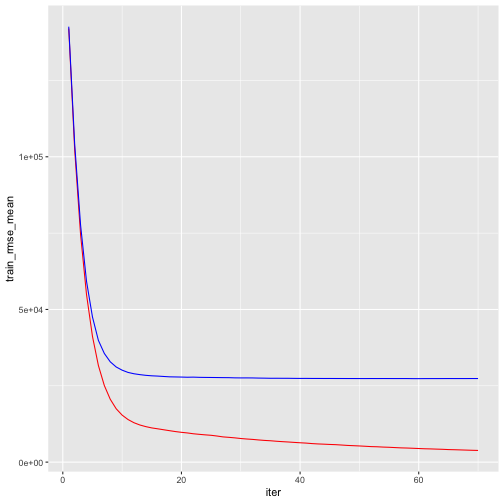
將模型結果印出。最佳迭代數(所需模型數)為1260。
|
1 |
gbm.perf(object = gbm.fit2, method = "cv") |
|
1 2 |
## [1] 1260 |
「grid search自動化tuning」
因為手動調整參數是沒效率的,我們來建立hyperparameters grid並自動套用grid search。
|
1 2 3 4 5 6 7 8 9 10 11 12 |
# create hyperparameter grid hyper_grid shrinkage = c(.01, .1, .3), # 學習步伐 interaction.depth = c(1, 3, 5), # 模型切割數 n.minobsinnode = c(5, 10, 15), # 節點最小觀測值個數 bag.fraction = c(.65, .8, 1), # 使用隨機梯度下降( optimal_trees = 0, # 儲存最適模型樹的欄位 min_RMSE = 0 # 儲存最小均方差的欄位 ) # total number of combinations nrow(hyper_grid) |
|
1 2 |
## [1] 81 |
我們一一測試以上81種超參數排列組合的效果,並指定使用5000個樹模型。
另外,為了降低執行的時間,有別於使用cross validation,我們改使用75%的訓練資料,使用剩下的25%的資料來進行OOB評估效果。需要特別注意的是,當使用train.fraction參數時,模型會直接使用前XX %的資料來使用,因此需要確保說資料是隨機排列的。
先將資料進行隨機排列處理。
|
1 2 3 |
# randomize data random_index random_ames_train |
開始執行grid search
|
1 2 3 4 5 6 7 8 9 10 11 12 13 14 15 16 17 18 19 20 21 22 23 24 25 |
# grid search for(i in 1:nrow(hyper_grid)) { # reproducibility set.seed(123) # train model gbm.tune formula = Sale_Price ~ ., distribution = "gaussian", data = random_ames_train, n.trees = 5000, # 使用5000個樹模型 interaction.depth = hyper_grid$interaction.depth[i], shrinkage = hyper_grid$shrinkage[i], n.minobsinnode = hyper_grid$n.minobsinnode[i], bag.fraction = hyper_grid$bag.fraction[i], train.fraction = .75, # 使用75%的訓練資料,並用剩餘資料做OOB成效評估/驗證 n.cores = NULL, # will use all cores by default verbose = FALSE ) # 將每個GBM模型最小的模型代號和對應的驗證均方誤差(valid RMSE)回傳到 hyper_grid$optimal_trees[i] hyper_grid$min_RMSE[i] } |
將每種參數組合的結果,依照RMSE由小到大排列,並取出排名前10的模型,查看參數組合細節。
|
1 2 3 |
hyper_grid %>% dplyr::arrange(min_RMSE) %>% head(10) |
|
1 2 3 4 5 6 7 8 9 10 11 12 13 14 15 16 17 18 19 20 21 22 23 |
## shrinkage interaction.depth n.minobsinnode bag.fraction optimal_trees ## 1 0.01 5 5 0.65 3867 ## 2 0.01 5 5 0.80 4209 ## 3 0.01 5 5 1.00 4281 ## 4 0.10 3 10 0.80 489 ## 5 0.01 3 5 0.80 4777 ## 6 0.01 3 10 0.80 4919 ## 7 0.01 3 5 0.65 4997 ## 8 0.01 5 10 0.80 4123 ## 9 0.01 5 10 0.65 4850 ## 10 0.01 3 10 1.00 4794 ## min_RMSE ## 1 16647.87 ## 2 16960.78 ## 3 17084.29 ## 4 17093.77 ## 5 17121.26 ## 6 17139.59 ## 7 17139.88 ## 8 17162.60 ## 9 17247.72 ## 10 17353.36 |
我們可以看到以下幾點:
- 最佳模型的最小RMSE(17K),較先前的RMSE(23K)降低了有6K左右。
- 前十的模型的學習步伐都小於0.3,表示較小的學習步伐在尋找最小誤差的模型效果是不錯的。
- 前十的模型都選用>1切割數的樹模型,。
- 十個模型有8個模型都使用bag.fraction < 1的隨機梯度下降(即使用<100%的訓練資料集進行每個模型的訓練),這將有助於避免overfitting以及陷在loss function gradient的局部最小最大值。
- 前十的模型中,也沒有使用採用節點觀測數大於等於15者。因為較小觀測數的節點較能捕捉到更多特徵。
- 部分參數組合所使用的最佳迭代數(總樹模型數)都很接近5000個。下次執行grid search時或許可以考慮增大樹模型數。
根據以上測試,我們已更接近最適的參數組合區間,我們此時在此聚焦範圍內再一次執行81種超參數組合的最佳模型搜尋。
|
1 2 3 4 5 6 7 8 9 10 11 12 |
# 根據上一部的結果,調整參數區間與數值 hyper_grid_2 shrinkage = c(.01, .05, .1), # 聚焦更小的學習步伐 interaction.depth = c(3, 5, 7), #聚焦>1的切割數 n.minobsinnode = c(5, 7, 10), # 聚焦更小的節點觀測值數量 bag.fraction = c(.65, .8, 1), # 不變 optimal_trees = 0, # a place to dump results min_RMSE = 0 # a place to dump results ) # total number of combinations nrow(hyper_grid_2) |
|
1 2 |
## [1] 81 |
我們再一次的用for loop迴圈執行以上81種超參數組合的模型,找出每一次最適的模型與對應的最小誤差。
|
1 2 3 4 5 6 7 8 9 10 11 12 13 14 15 16 17 18 19 20 21 22 23 24 25 |
# grid search for(i in 1:nrow(hyper_grid_2)) { # reproducibility set.seed(123) # train model gbm.tune formula = Sale_Price ~ ., distribution = "gaussian", data = random_ames_train, n.trees = 6000, interaction.depth = hyper_grid_2$interaction.depth[i], shrinkage = hyper_grid_2$shrinkage[i], n.minobsinnode = hyper_grid_2$n.minobsinnode[i], bag.fraction = hyper_grid_2$bag.fraction[i], train.fraction = .75, # 使用剩餘的25%資料估計OOB誤差 n.cores = NULL, # will use all cores by default verbose = FALSE ) # add min training error and trees to grid hyper_grid_2$optimal_trees[i] hyper_grid_2$min_RMSE[i] } |
檢視結果
|
1 2 3 |
hyper_grid_2 %>% dplyr::arrange(min_RMSE) %>% head(10) |
|
1 2 3 4 5 6 7 8 9 10 11 12 13 14 15 16 17 18 19 20 21 22 23 |
## shrinkage interaction.depth n.minobsinnode bag.fraction ## 1 0.01 5 5 0.65 ## 2 0.01 7 5 0.65 ## 3 0.05 5 5 0.65 ## 4 0.01 7 5 0.80 ## 5 0.01 7 7 0.65 ## 6 0.05 5 10 0.80 ## 7 0.01 5 5 0.80 ## 8 0.01 3 7 0.80 ## 9 0.01 5 7 0.65 ## 10 0.01 5 7 0.80 ## optimal_trees min_RMSE ## 1 3867 16647.87 ## 2 2905 16782.26 ## 3 640 16783.13 ## 4 4193 16833.74 ## 5 3275 16906.53 ## 6 958 16933.12 ## 7 4209 16960.78 ## 8 5813 16998.79 ## 9 4798 17003.94 ## 10 4753 17004.20 |
本次結果與上一次結果十分類似。最佳模型和上一次選出的最佳模型是一樣的(相同的參數排列組合),RMSE約是17K。
一旦找到最佳模型,我們則可使用該參數組合來train一個模型。也因為最佳模型約收斂在僅1634個樹模型,我們可以 訓練一個由1634個樹模型所組成的cross validation模型(使用CV來提供更穩健的誤差估計值)。
|
1 2 3 4 5 6 7 8 9 10 11 12 13 14 15 16 17 18 19 20 |
# for reproducibility set.seed(123) system.time( # train GBM model gbm.fit.final formula = Sale_Price ~ ., distribution = "gaussian", data = ames_train, n.trees = 1634, interaction.depth = 5, shrinkage = 0.05, n.minobsinnode = 7, bag.fraction = .8, train.fraction = 1, # 如果使用 cv.folds = 4, # 有別於使用OOB估計誤差,我們估計更穩健的CV誤差 n.cores = NULL, # will use all cores by default verbose = FALSE ) ) |
|
1 2 3 |
## user system elapsed ## 18.394 0.617 49.558 |
最佳模型的cv誤差如下(22K)。
|
1 |
sqrt(min(gbm.fit.final$cv.error)) # 必須是模型參數cv.folds > 1 才會回傳cv.error |
|
1 2 |
## [1] 22165.11 |
視覺化
variable importance
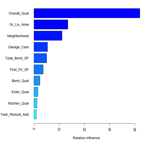
執行完最後的最佳模型後(gbm.fit.final),我們會想要看對目標變數sale price來說最有影響力的解釋變數有哪些,以捕捉模型的「可解釋性」。我們可以使用summary()函數來回傳gmb模型中最具影響力的解釋變數清單(data frame & plot)。並可以使用gbm模型summary函式中的cBars參數來指定要顯示的解釋變數清單數(根據影響力排名)。預設使用相對影響力來計算變數重要性。以下說明計算變數重要性的兩個方法:
- method = relative.influence: 每棵樹在進行節點分割時,gbm會計算每個變數作為切點,切割後對模型誤差所帶來的改善(回歸模型的話就是MSE)。gbm於是會平均每個變數在不同樹模型的誤差改善值,當作變數影響力。具有越高平均誤差降低值得變數即被視作最具影響力的變數。
- method = permutation.test.gbm: 模型會隨機置換(一次一個)不同預測變數,來計算個別變數的對預測性能的改善(使用所有training data),並平均每個變數在不同樹模型對正確率造成的改變量。具有越高正確率改變量的預測變數越具重要性。
|
1 2 3 4 5 6 7 8 9 |
par(mar = c(5, 8, 1, 1)) # S3 method for class 'gbm' summary( gbm.fit.final, # gbm object cBars = 10, # the number of bars to draw. length(object$var.names) plotit = TRUE, # an indicator as to whether the plot is generated.defult TRUE. method = relative.influence, # The function used to compute the relative influence. 亦可使用permutation.test.gbm las = 2 ) |
|
1 2 3 4 5 6 7 8 9 10 11 12 13 14 15 16 17 18 19 20 21 22 23 24 25 26 27 28 29 30 31 32 33 34 35 36 37 38 39 40 41 42 43 44 45 46 47 48 49 50 51 52 53 54 55 56 57 58 59 60 61 62 63 64 65 66 67 68 69 70 71 72 73 74 75 76 77 78 79 80 81 82 |
## var rel.inf ## Overall_Qual Overall_Qual 4.199240e+01 ## Gr_Liv_Area Gr_Liv_Area 1.343609e+01 ## Neighborhood Neighborhood 1.111899e+01 ## Garage_Cars Garage_Cars 5.374303e+00 ## Total_Bsmt_SF Total_Bsmt_SF 5.031406e+00 ## First_Flr_SF First_Flr_SF 3.641743e+00 ## Bsmt_Qual Bsmt_Qual 2.365967e+00 ## Exter_Qual Exter_Qual 1.559647e+00 ## Kitchen_Qual Kitchen_Qual 1.210399e+00 ## Year_Remod_Add Year_Remod_Add 9.800489e-01 ## MS_SubClass MS_SubClass 9.168515e-01 ## Fireplace_Qu Fireplace_Qu 7.900484e-01 ## Mas_Vnr_Area Mas_Vnr_Area 7.480704e-01 ## Lot_Area Lot_Area 7.181146e-01 ## Bsmt_Unf_SF Bsmt_Unf_SF 7.036017e-01 ## Second_Flr_SF Second_Flr_SF 6.564021e-01 ## Garage_Area Garage_Area 5.812072e-01 ## Screen_Porch Screen_Porch 5.697864e-01 ## Bsmt_Exposure Bsmt_Exposure 5.447030e-01 ## Overall_Cond Overall_Cond 5.149690e-01 ## BsmtFin_Type_1 BsmtFin_Type_1 5.136834e-01 ## Full_Bath Full_Bath 4.517156e-01 ## Lot_Frontage Lot_Frontage 4.308841e-01 ## Latitude Latitude 4.021943e-01 ## Sale_Condition Sale_Condition 3.736402e-01 ## Garage_Type Garage_Type 3.400862e-01 ## Bsmt_Full_Bath Bsmt_Full_Bath 2.830678e-01 ## Garage_Finish Garage_Finish 2.794122e-01 ## Open_Porch_SF Open_Porch_SF 2.731140e-01 ## Exterior_1st Exterior_1st 2.449858e-01 ## Fireplaces Fireplaces 2.446628e-01 ## Sale_Type Sale_Type 2.083020e-01 ## Year_Built Year_Built 2.060348e-01 ## Central_Air Central_Air 1.895762e-01 ## Exterior_2nd Exterior_2nd 1.791393e-01 ## TotRms_AbvGrd TotRms_AbvGrd 1.624508e-01 ## Wood_Deck_SF Wood_Deck_SF 1.619419e-01 ## Mo_Sold Mo_Sold 1.556240e-01 ## Condition_1 Condition_1 1.555862e-01 ## Garage_Cond Garage_Cond 1.433484e-01 ## Functional Functional 1.195756e-01 ## Land_Contour Land_Contour 1.176260e-01 ## Longitude Longitude 1.099157e-01 ## Heating_QC Heating_QC 7.996284e-02 ## Year_Sold Year_Sold 7.732664e-02 ## Roof_Matl Roof_Matl 6.581906e-02 ## House_Style House_Style 5.653741e-02 ## Mas_Vnr_Type Mas_Vnr_Type 4.764729e-02 ## Bedroom_AbvGr Bedroom_AbvGr 4.542366e-02 ## Lot_Config Lot_Config 3.928406e-02 ## Paved_Drive Paved_Drive 3.815510e-02 ## BsmtFin_Type_2 BsmtFin_Type_2 3.573880e-02 ## Roof_Style Roof_Style 3.492513e-02 ## Bsmt_Cond Bsmt_Cond 3.320548e-02 ## Land_Slope Land_Slope 3.191664e-02 ## Exter_Cond Exter_Cond 3.036215e-02 ## MS_Zoning MS_Zoning 3.016913e-02 ## Enclosed_Porch Enclosed_Porch 2.361207e-02 ## Alley Alley 1.860542e-02 ## Condition_2 Condition_2 1.829088e-02 ## Half_Bath Half_Bath 1.622231e-02 ## Three_season_porch Three_season_porch 1.091252e-02 ## Foundation Foundation 1.039571e-02 ## Low_Qual_Fin_SF Low_Qual_Fin_SF 8.975948e-03 ## BsmtFin_SF_2 BsmtFin_SF_2 8.747153e-03 ## Fence Fence 7.868905e-03 ## Lot_Shape Lot_Shape 5.645516e-03 ## Electrical Electrical 4.850525e-03 ## Heating Heating 4.405392e-03 ## Garage_Qual Garage_Qual 3.845332e-03 ## BsmtFin_SF_1 BsmtFin_SF_1 2.902816e-03 ## Misc_Val Misc_Val 2.321802e-03 ## Bsmt_Half_Bath Bsmt_Half_Bath 2.263392e-03 ## Street Street 1.157860e-03 ## Bldg_Type Bldg_Type 4.970819e-04 ## Misc_Feature Misc_Feature 4.236315e-04 ## Pool_QC Pool_QC 1.575743e-04 ## Pool_Area Pool_Area 9.720817e-05 ## Utilities Utilities 0.000000e+00 ## Kitchen_AbvGr Kitchen_AbvGr 0.000000e+00 |
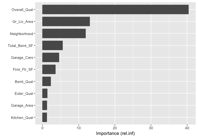
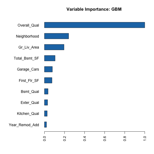
另外一個方式,就是使用vip套件(variable importance plot)的vip函式,會回傳ggplot形式的重要變數圖表。 為兩個解釋集成樹的兩大重要解釋指標),是許多機器學習模型常用的變數重要性繪圖框架。
|
1 2 |
# install.packages('vip') vip::vip(gbm.fit.final) |
Partial dependence plots
一旦識別出最重要的幾個變數後,下一步就是去了解當解釋變數變動時,目標變數是如何變動的(即marginal effects,邊際效果,每變動一單位解釋變數時,對目標變數的影響)。我們可以使用partial dependence plots(PDPs)和individual conditional expectation(ICE)曲線。
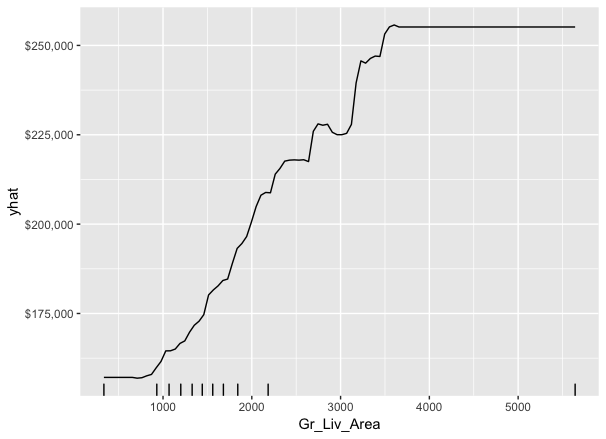
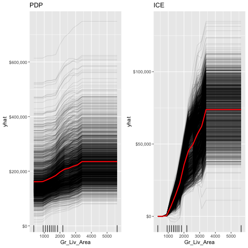
- PDPs: 繪製特定變數邊際變動造成的平均目標預測值的變動。比如說,下圖繪製了預測變數Gr_Liv_Area邊際變動(控制其他變數不變的情況下)對平均目標預測銷售金額(avg. sale price_的影響。下圖PDPs描述隨著房屋基底的面積邊際增加,平均銷售價格增加的變化。
|
1 2 3 4 5 6 7 8 |
gbm.fit.final %>% partial(object = .,# A fitted model object of appropriate class (e.g., "gbm", "lm", "randomForest", "train", etc.). pred.var = "Gr_Liv_Area", n.trees = gbm.fit.final$n.trees, # 如果是gbm的話,需指定模型所使用樹個數 grid.resolution = 100) %>% # The autplot function can be used to produce graphics based on ggplot2 autoplot(rug = TRUE, train = ames_train) + # plotPartial()不支援gbm scale_y_continuous(labels = scales::dollar) # 因為是使用ggplot基礎繪圖,故可以使用ggplot相關圖層來調整 |
拆解步驟1: 先檢視沒有繪圖(plot = FALSE)的所回傳的data.frame。在一些例子中,使用partial根據object來擷取training data是困難的,此時便會出現錯誤訊息要求使用者透過train參數提供訓練資料集。但絕大部分的時候,partial會預設擷取當下環境下訓練object所使用的訓練資料集,所以很重要的事,在執行partial之前不行改變到訓練資料集的變數內容,而此問題可透過明確指定train參數所對應的訓練資料集而解決。
|
1 2 3 4 5 6 |
partialDf object = gbm.fit.final,pred.var = "Gr_Liv_Area", n.trees = gbm.fit.final$n.trees, grid.resolution = 100, train = ames_train) partialDf |
|
1 2 3 4 5 6 7 8 9 10 11 12 13 14 15 16 17 18 19 20 21 22 23 24 25 26 27 28 29 30 31 32 33 34 35 36 37 38 39 40 41 42 43 44 45 46 47 48 49 50 51 52 53 54 55 56 57 58 59 60 61 62 63 64 65 66 67 68 69 70 71 72 73 74 75 76 77 78 79 80 81 82 83 84 85 86 87 88 89 90 91 92 93 94 95 96 97 98 99 100 101 102 |
## Gr_Liv_Area yhat ## 1 334 156956.9 ## 2 387 156956.9 ## 3 441 156956.9 ## 4 494 156956.9 ## 5 548 156956.9 ## 6 602 156956.9 ## 7 655 156956.9 ## 8 709 156660.6 ## 9 762 156755.5 ## 10 816 156871.1 ## 11 870 156871.1 ## 12 923 158251.7 ## 13 977 161056.8 ## 14 1031 163112.1 ## 15 1084 163138.2 ## 16 1138 163214.8 ## 17 1191 166534.4 ## 18 1245 166987.2 ## 19 1299 169077.6 ## 20 1352 170758.6 ## 21 1406 172776.0 ## 22 1459 174681.8 ## 23 1513 181046.8 ## 24 1567 182290.3 ## 25 1620 185044.8 ## 26 1674 185035.8 ## 27 1728 186329.2 ## 28 1781 189560.9 ## 29 1835 192374.4 ## 30 1888 193609.3 ## 31 1942 194775.0 ## 32 1996 200759.0 ## 33 2049 202826.8 ## 34 2103 206586.7 ## 35 2156 207502.2 ## 36 2210 207502.2 ## 37 2264 209486.0 ## 38 2317 212637.8 ## 39 2371 214445.4 ## 40 2425 214863.0 ## 41 2478 215367.1 ## 42 2532 215404.3 ## 43 2585 215404.3 ## 44 2639 215571.6 ## 45 2693 226433.3 ## 46 2746 225632.2 ## 47 2800 225849.6 ## 48 2853 223628.9 ## 49 2907 219924.6 ## 50 2961 218770.4 ## 51 3014 218770.4 ## 52 3068 218770.4 ## 53 3122 227327.1 ## 54 3175 229537.3 ## 55 3229 235917.9 ## 56 3282 241038.0 ## 57 3336 240301.2 ## 58 3390 243415.0 ## 59 3443 243127.7 ## 60 3497 246930.9 ## 61 3550 246930.9 ## 62 3604 246930.9 ## 63 3658 246930.9 ## 64 3711 246930.9 ## 65 3765 246930.9 ## 66 3819 246930.9 ## 67 3872 246930.9 ## 68 3926 246930.9 ## 69 3979 246930.9 ## 70 4033 246930.9 ## 71 4087 246930.9 ## 72 4140 246930.9 ## 73 4194 246930.9 ## 74 4247 246930.9 ## 75 4301 246930.9 ## 76 4355 246930.9 ## 77 4408 246930.9 ## 78 4462 246930.9 ## 79 4516 246930.9 ## 80 4569 246930.9 ## 81 4623 246930.9 ## 82 4676 246930.9 ## 83 4730 246930.9 ## 84 4784 246930.9 ## 85 4837 246930.9 ## 86 4891 246930.9 ## 87 4944 246930.9 ## 88 4998 246930.9 ## 89 5052 246930.9 ## 90 5105 246930.9 ## 91 5159 246930.9 ## 92 5213 246930.9 ## 93 5266 246930.9 ## 94 5320 246930.9 ## 95 5373 246930.9 ## 96 5427 246930.9 ## 97 5481 246930.9 ## 98 5534 246930.9 ## 99 5588 246930.9 ## 100 5642 246930.9 |
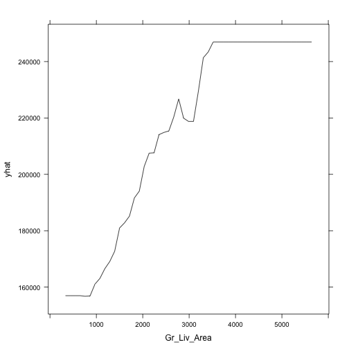
亦可使用plot = TRUE將以上結果繪出。(不是ggplot2)
但其實比較推薦保留plot = FALSE,將partial回傳結果先儲存。這樣的好處在於繪圖上會更有彈性,當預設繪圖結果不足夠時,不需要重新執行partial()。
|
1 |
partial(gbm.fit.final, train = ames_train, pred.var = 'Gr_Liv_Area',n.trees = gbm.fit.final$n.trees, plot = TRUE) |
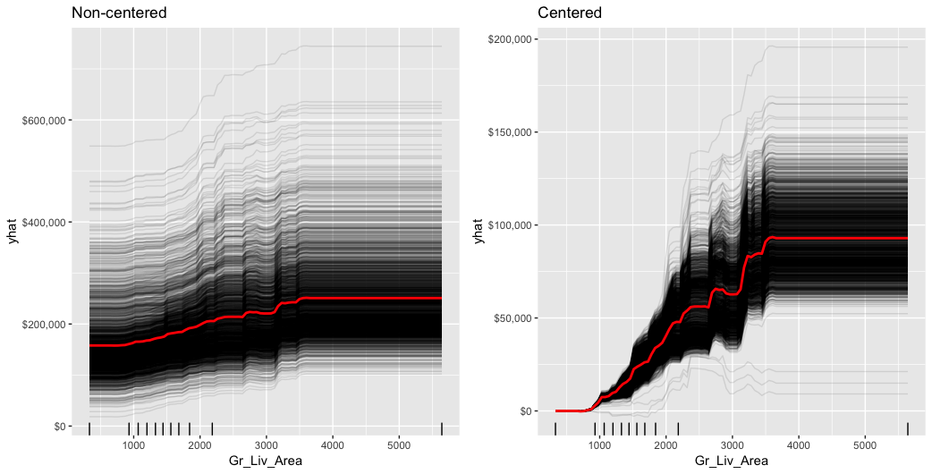
- ICE curves: 是PDPs圖的延伸。與PDPs圖不同的地方在於,PDPs是繪製每個解釋變數邊際變動所造成的「平均」目標數值的變化(平均所有觀測值),而ICE curves則是繪製「每個」解釋變數邊際變動對所有觀測值的目標數值的變動。下面分別呈現了regular ICE曲線圖(左)和centered ICE曲線圖(右)。當曲線有很寬廣的截距且彼此疊在一起,很難辨別感興趣的預測變數邊際變動所造成的回應變數變動量的異質性。而centered ICE曲線,則能強調結果中的異質性。以下regular ICE圖顯示,當Gr_Liv_Area增加時,大部分的觀測值的目標變數變化具有共通趨勢,而centered ICE圖則凸顯部分與共通趨勢不一致的觀察值變化圖。
|
1 2 3 4 5 6 7 8 9 10 |
ice1 % partial( pred.var = "Gr_Liv_Area", n.trees = gbm.fit.final$n.trees, grid.resolution = 100, ice = TRUE # 當ice = TRUE或給定pred.fun參數,會回傳使用newdata替每個觀測值預測的結果 ) %>% autoplot(rug = TRUE, train = ames_train, alpha = .1) + # alpha參數只在ICE curves繪製上有效 ggtitle("Non-centered") + scale_y_continuous(labels = scales::dollar) |
|
1 2 3 4 5 6 7 8 9 10 |
ice2 % partial( pred.var = "Gr_Liv_Area", n.trees = gbm.fit.final$n.trees, grid.resolution = 100, ice = TRUE ) %>% autoplot(rug = TRUE, train = ames_train, alpha = .1, center = TRUE) + ggtitle("Centered") + scale_y_continuous(labels = scales::dollar) |
|
1 |
gridExtra::grid.arrange(ice1, ice2, nrow = 1) |
LIME
LIME是一種新程序幫助我們了解,單一觀察值的預測目標值是如何產生的。對gbm物件使用lime套件,我們需要定義模型類型model type和預測方法prediction methods。
|
1 2 3 4 5 6 7 8 |
model_type.gbm return("regression") } predict_model.gbm pred return(as.data.frame(pred)) } |
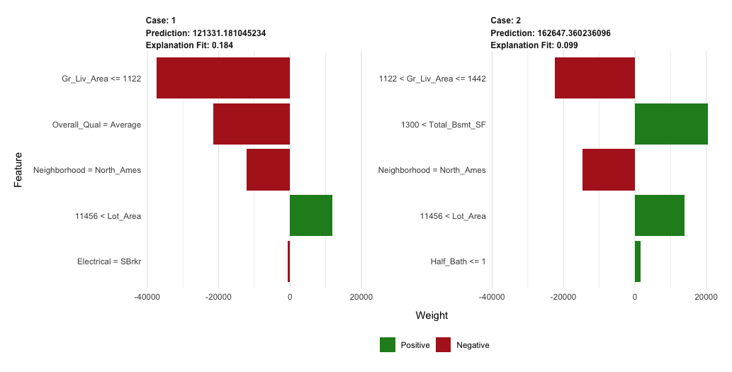
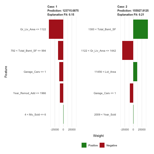
以下我們便挑選兩個觀測值來檢視其預測目標值是如何產生的。
結果包括預測目標值(分別為case1: 127K case2: 159K)、局部模型配適(兩者的局部配飾都太好)、以及對不同觀測值來說,對目標變數最具影響力的特徵變數。
|
1 2 3 4 5 6 7 8 9 10 11 12 13 |
# get a few observations to perform local interpretation on local_obs # apply LIME explainer x=ames_train, # The training data used for training the model that should be explained. model = gbm.fit.final # The model whose output should be explained ) # 一旦使用lime()創建好了explainer,則可將explainer用作解釋模型作用在新觀察值的結果 explanation explainer = explainer, n_features = 5 # The number of features to use for each explanation. ) |
|
1 |
plot_features(explanation = explanation) |
Predicting
一旦決定好最佳的模型後,便使用模型來預測新的資料集(ames_test)。跟大部分模型一樣,我們可以使用predict()函數,只不過我們需要指定所需要的樹模型個數(可參考?predict.gbm之說明)。我們可以觀察到,測試資料集所得到的RMSE跟我們得到的最佳gbm模型的RMSE(22K)是差不多的。
|
1 2 3 4 5 |
# predict values for test data pred # results caret::RMSE(pred, ames_test$Sale_Price) |
|
1 2 |
## [1] 19686.42 |
xgboost
xgboost套件提供一個Extreme Gradient Boosting的R API,可以具效率地去執行gradient boosting framework(約比gbm套件快上10倍)。xgboost文件的知識庫有豐富的資訊。亦可參考非常完整的參數tuning教學文章。xgboost套件一直以來在kaggle data mining競賽上是滿受歡迎且成功的演算法套件。
xgboost幾個特色包括:
- 提供內建的k-fold cross validation
- 隨機GBM,兼具column和row的抽樣(per split and per tree),以達到更好的一般性(避免過度擬合)。
- 包括高效的線性模型求解器和樹學習演算法。
- 單一機器上的平行運算。
- 支援多個目標函數,包括回歸regression,分類classification,和排序ranking。
- 該套件被設計為有延展性的(extensible),因此使用者可以自己定義自己的目標函式(objectives)。
- Apache 2.0 License
基本的xgboost實作
xgboost 只能在都是「數值變數的矩陣」下運作(由於在空間中表示點的位置,所有特徵值須為數值)。因此,我們必須先將數據進行編碼轉換。
一般來說編碼類別變數有兩種方式,分別為Label Encoding和one-hot encoding,通常前者會衍伸出編碼後的數值變成有順序意義在的問題,以及在空間維度中代表不同距離的意義之問題,故通常最常使用one-hot encoding法是最適合的,來使類別變數中三個屬性在空間中距離原點的距離是相同的(*但必須注意的是,one-hot encoding只適用在類別種類少的情況,如果種類過多,過多展開的維度會衍伸出其他問題)。
在R中有幾個執行one-hot encoding的方式,包括Matrix::sparse.model.matrix, caret::dummyVars,但我們這邊會使用vtreat套件。vtreat是一個強大的資料前處理套件,且有助於處理因遺失值、或新資料中才新冒出的類別資料級別(原本不為訓練資料類別變數中的選項)等因素而造成的問題。然而vtreat在使用上不是很直覺。本篇學習筆記在此不會說明太多vtreat的功能,如需要了解可先參考連結1,連結2和連結3。
以下使用vtreat將training & testing資料即重新one-hot encoding編碼。
|
1 2 3 4 5 6 7 8 9 10 11 12 13 14 15 16 17 18 19 |
# variable names features # Create the treatment plan from the training data treatplan # Get the "clean" variable names from the scoreFrame new_vars % magrittr::use_series(scoreFrame) %>% dplyr::filter(code %in% c("clean", "lev")) %>% magrittr::use_series(varName) # Prepare the training data features_train % as.matrix() response_train # Prepare the test data features_test % as.matrix() response_test |
編碼後的維度個數
|
1 |
dim(features_train) |
|
1 2 |
## [1] 2051 348 |
|
1 |
dim(features_test) |
|
1 2 |
## [1] 879 348 |
xgboost提供不同的訓練函數(像是xgb.train,xgb.cv)。而我們這邊會使用能夠進行cross-validation的xgb.cv。以下我們訓練一個使用5-fold cv且使用1000棵樹的xgb模型。xgb.cv中有許多可調整的參數(基本的參數都跟xgb.train是一樣的),幾個比較常出現的參數(與其預設值)分別為以下:
- data: 只允許數值型矩陣,如xgb.DMatrix, matrix, dgCMartirx類型。
- nrounds: 模型所使用的樹個數(迭代數)。
- nfold: 將投入的data參數值(在此處為訓練資料集),隨機切割(partition)為n等分的子樣本。
- params: list(),參數list。常用的參數包括:
- objective : 目標函數(亦可使用params = list()進行參數指定)。常用的目標函數包括:
- reg:linear : 線性迴歸
- binary:logistic : 分類用的羅吉斯迴歸
- eta: learning rate,學習步伐(default為0.3)
- max_depth: tree depth, 樹模型的深度(default為6)
- min_child_weight: minimum node size,最小節點個數值(default為1)
- subsample: percentage of training data to sample for each tree (就如同gbm套件中的bag.fraction參數),每棵樹模型將抽樣使用多少比例的訓練資料集(default: 100% -> 沒有OOB sample),用來避免overfitting,亦可加快運算(分析較少的資料)。
其中cross-validation會執行nrounds次,每次迭代中,nfold個子樣本都會輪流作為驗證資料集,來驗證nfold-1子集合所訓練出的模型。
|
1 2 3 4 5 6 7 8 9 10 11 12 13 |
# reproducibility set.seed(123) system.time( xgb.fit1 data = features_train, label = response_train, nrounds = 1000, nfold = 5, objective = "reg:linear", # for regression models verbose = 0 # silent,不要顯示詳細資訊 ) ) |
|
1 2 3 |
## user system elapsed ## 234.376 2.540 244.823 |
檢視每次迭代的cross-validation的結果。分別會有訓練資料集的平均RMSE,和測試資料集的平均RMSE,希望兩者越接近越好。
|
1 |
print(xgb.fit1,verbose = TRUE) |
|
1 2 3 4 5 6 7 8 9 10 11 12 13 14 15 16 17 18 19 20 21 22 23 |
## ##### xgb.cv 5-folds ## call: ## xgb.cv(data = features_train, nrounds = 1000, nfold = 5, label = response_train, ## verbose = 0, objective = "reg:linear") ## params (as set within xgb.cv): ## objective = "reg:linear", silent = "1" ## callbacks: ## cb.evaluation.log() ## niter: 1000 ## evaluation_log: ## iter train_rmse_mean train_rmse_std test_rmse_mean test_rmse_std ## 1 1.420236e+05 850.15595494 142612.98 4504.553 ## 2 1.023304e+05 645.18845214 104198.60 4628.932 ## 3 7.443451e+04 535.78249514 77533.40 4635.993 ## 4 5.484559e+04 468.37246662 59185.94 4420.339 ## 5 4.118994e+04 386.94999310 47545.03 4452.632 ## --- ## 996 4.831320e-02 0.01131165 27373.21 3243.812 ## 997 4.831320e-02 0.01131165 27373.21 3243.812 ## 998 4.831320e-02 0.01131165 27373.21 3243.812 ## 999 4.831320e-02 0.01131165 27373.21 3243.811 ## 1000 4.831320e-02 0.01131165 27373.21 3243.812 |
檢視回傳xbg.fit1物件的屬性(attributes)。
|
1 |
attributes(xgb.fit1) |
|
1 2 3 4 5 6 7 8 |
## $names ## [1] "call" "params" "callbacks" ## [4] "evaluation_log" "niter" "nfeatures" ## [7] "folds" ## ## $class ## [1] "xgb.cv.synchronous" |
回傳的xgb.fit1物件包含很多重要資訊。特別像是我們可以擷取xgb.fit1$evaluation_log來觀察發生在訓練資料集和測試資料集的最小的RMSE和最適的樹數量(跟print(xgb.fit1)效果一樣),以及cross-validation error。
|
1 |
xgb.fit1$evaluation_log |
|
1 2 3 4 5 6 7 8 9 10 11 12 13 14 15 16 17 18 19 20 21 22 23 24 25 |
## iter train_rmse_mean train_rmse_std test_rmse_mean ## 1: 1 1.420236e+05 850.15595494 142612.98 ## 2: 2 1.023304e+05 645.18845214 104198.60 ## 3: 3 7.443451e+04 535.78249514 77533.40 ## 4: 4 5.484559e+04 468.37246662 59185.94 ## 5: 5 4.118994e+04 386.94999310 47545.03 ## --- ## 996: 996 4.831320e-02 0.01131165 27373.21 ## 997: 997 4.831320e-02 0.01131165 27373.21 ## 998: 998 4.831320e-02 0.01131165 27373.21 ## 999: 999 4.831320e-02 0.01131165 27373.21 ## 1000: 1000 4.831320e-02 0.01131165 27373.21 ## test_rmse_std ## 1: 4504.553 ## 2: 4628.932 ## 3: 4635.993 ## 4: 4420.339 ## 5: 4452.632 ## --- ## 996: 3243.812 ## 997: 3243.812 ## 998: 3243.812 ## 999: 3243.811 ## 1000: 3243.812 |
我們找出使得訓練和測試誤差最小的迭代數(模型所使用的樹個數),以及所對應的RMSE。由下表所示,訓練誤差持續下降,並約在924棵樹時逼近為零(0.048)。然而,交叉驗證誤差約在60棵樹左右達到最小RMSE(約27K)。
|
1 2 3 4 5 6 7 8 |
# get number of trees that minimize error xgb.fit1$evaluation_log %>% dplyr::summarise( ntrees.train = which(train_rmse_mean == min(train_rmse_mean))[1], rmse.train = min(train_rmse_mean), ntrees.test = which(test_rmse_mean == min(test_rmse_mean))[1], rmse.test = min(test_rmse_mean) ) |
|
1 2 3 |
## ntrees.train rmse.train ntrees.test rmse.test ## 1 924 0.0483002 60 27337.79 |
|
1 2 |
## ntrees.train rmse.train ntrees.test rmse.test ## 1 965 0.5022836 60 27572.31 |
將詳細xgboost模型迭代資訊繪出如下,紅色線代表訓練誤差,藍色線表示交叉驗證誤差。
|
1 2 3 4 |
# plot error vs number trees ggplot(xgb.fit1$evaluation_log) + geom_line(aes(iter, train_rmse_mean), color = "red") + geom_line(aes(iter, test_rmse_mean), color = "blue") |
一個xbm.cv滿不錯的功能就是early stopping。該功能讓我們可在cross validation error在連續第n棵樹不再下降的情況下,告訴函式該停止。以上面的例子來說,我們可以設定當cv error在連續10個樹模型(迭代)沒有下降時停止迭代(early_stopping_rounds = 10)。該功能有助於加速下一個tuning校正過程。
|
1 2 3 4 5 6 7 8 9 10 11 12 |
# reproducibility set.seed(123) xgb.fit2 data = features_train, label = response_train, nrounds = 1000, nfold = 5, objective = "reg:linear", # for regression models verbose = 0, # silent, early_stopping_rounds = 10 # stop if no improvement for 10 consecutive trees ) |
將迭代的過程細節繪出:
|
1 2 3 4 |
# plot error vs number trees ggplot(xgb.fit2$evaluation_log) + geom_line(aes(iter, train_rmse_mean), color = "red") + geom_line(aes(iter, test_rmse_mean), color = "blue") |
Tuning
要tune XGBoost模型,我們會傳入一個parameters的list物件給params參數。幾個最常見的參數如下:
- eta : 控制學習步伐
- max_depth: 樹的深度
- min_child_weight: 末梢節點的最小觀測值個數
- subsample: 每棵樹模型所抽樣訓練資料集的比例
- colsample_bytrees: 每棵樹模型所抽樣的欄位數目
舉例來說,如果想要指定特定參數值,我們可以將上面的模型設定重新編輯如下:
|
1 2 3 4 5 6 7 8 9 10 11 12 13 14 15 16 17 18 19 20 21 22 23 24 25 |
# create parameter list params eta = .1, max_depth = 5, min_child_weight = 2, subsample = .8, colsample_bytree = .9 ) # reproducibility set.seed(123) # train model system.time( xgb.fit3 params = params, data = features_train, label = response_train, nrounds = 1000, nfold = 5, objective = "reg:linear", # for regression models verbose = 0, # silent, early_stopping_rounds = 10 # stop if no improvement for 10 consecutive trees ) ) |
|
1 2 3 |
## user system elapsed ## 39.185 0.124 39.446 |
|
1 2 3 4 5 6 7 8 |
# assess results xgb.fit3$evaluation_log %>% dplyr::summarise( ntrees.train = which(train_rmse_mean == min(train_rmse_mean))[1], rmse.train = min(train_rmse_mean), ntrees.test = which(test_rmse_mean == min(test_rmse_mean))[1], rmse.test = min(test_rmse_mean) ) |
|
1 2 3 |
## ntrees.train rmse.train ntrees.test rmse.test ## 1 220 5054.546 210 24159.13 |
想要執行更大型的search grid,我們可以使用和gbm相同的程序。先產生一個超參數hyperparameter search grid和儲存結果的欄位(最適樹模型個數與最小RMSE)。
以下我們創立一個4*4*4*3*3 = 576個參數排列組合的hyper grid。
|
1 2 3 4 5 6 7 8 9 10 11 12 |
# create hyperparameter grid hyper_grid eta = c(.01, .05, .1, .3), max_depth = c(1, 3, 5, 7), min_child_weight = c(1, 3, 5, 7), subsample = c(.65, .8, 1), colsample_bytree = c(.8, .9, 1), optimal_trees = 0, # a place to dump results min_RMSE = 0 # a place to dump results ) nrow(hyper_grid) |
|
1 2 |
## [1] 576 |
接著,我們使用迴圈一一去執行XGBoost模型套用不同參數組合的結果,並將結果指標儲存。(*這段程序耗時,約6小時以上)
|
1 2 3 4 5 6 7 8 9 10 11 12 13 14 15 16 17 18 19 20 21 22 23 24 25 26 27 28 29 30 31 32 33 34 35 |
# grid search for(i in 1:nrow(hyper_grid)) { # create parameter list params eta = hyper_grid$eta[i], max_depth = hyper_grid$max_depth[i], min_child_weight = hyper_grid$min_child_weight[i], subsample = hyper_grid$subsample[i], colsample_bytree = hyper_grid$colsample_bytree[i] ) # reproducibility set.seed(123) # train model xgb.tune params = params, data = features_train, label = response_train, nrounds = 5000, nfold = 5, objective = "reg:linear", # for regression models verbose = 0, # silent, early_stopping_rounds = 10 # stop if no improvement for 10 consecutive trees ) # add min training error and trees to grid hyper_grid$optimal_trees[i] hyper_grid$min_RMSE[i] } hyper_grid %>% dplyr::arrange(min_RMSE) %>% head(10) |
|
1 2 3 4 5 6 7 8 9 10 11 12 |
## eta max_depth min_child_weight subsample colsample_bytree optimal_trees min_RMSE ## 1 0.01 5 3 0.65 0.8 1501 23255.95 ## 2 0.05 5 5 0.80 0.9 486 23269.22 ## 3 0.01 5 3 0.65 0.9 1325 23373.22 ## 4 0.01 5 1 0.65 0.8 1257 23396.13 ## 5 0.05 5 7 0.65 1.0 508 23437.00 ## 6 0.01 3 3 0.65 1.0 2301 23457.89 ## 7 0.01 5 3 0.80 0.8 1488 23499.83 ## 8 0.01 7 3 0.65 0.8 1178 23519.53 ## 9 0.01 3 5 0.65 0.9 2274 23526.33 ## 10 0.05 5 7 0.80 0.8 401 23555.05 |
經過評估後,可能還會繼續測是幾個不同的參數組合,去找到最能影響模型成效的參數。這邊有一篇很棒的文章在討論tuning XGBoost的策略法。但為了簡短,在此我們即假設上述結果為globally最適的模型,並使用xgb.train()來配飾最終模型。(*xgboost)
|
1 2 3 4 5 6 7 8 9 10 11 12 13 14 15 16 17 18 |
# parameter list params eta = 0.01, max_depth = 5, min_child_weight = 5, subsample = 0.65, colsample_bytree = 1 ) # train final model xgb.fit.final params = params, data = features_train, label = response_train, nrounds = 1576, objective = "reg:linear", verbose = 0 ) |
Visualization
Variable importance
xgboost提供內建的變數重要性繪圖功能。首先,可以使用xgb.importance()函數建立一個重要矩陣(importance matrix)的data.table,然後再將這個重要矩陣(importance matrix)投入xgb.plot.importance()函數進行繪圖。
在重要性矩陣中,Gain, Cover, Frequency欄位分別代表三種不同的變數重要性衡量的方法(此為tree model的衡量指標,如果是linear mode,衡量指標則會是Weight(模型中的線性係數)和Class):
- Gain(貢獻度): 相應特徵對模型的相對貢獻度,計算特徵在模型中每棵樹的貢獻。其與gbm套件中的relative.influence是同意的。
- Cover(觀測值個數涵蓋率): 與該特徵相關的相對觀察值個數(%)。比如說,你有100個觀察值,4個特徵變數3棵樹,並假設feature 1是用來區分葉節點並在樹tree1, tree2, tree3有各有10,5,2個觀察值;於是feature 1的cover會被計算為10+5+2=17個觀察值。feature2 ~ feature4亦會計算各自的cover,並以該特徵涵蓋變數個數相對於所有特徵總涵蓋變數個數計算百分比。
- Frequency(出現在模型所有樹的相對次數):代表某特徵出現在模型中樹的相對次數百分比(%)。就上面的範例來說,假設feature 1分別在tree1, tree2,tree3的分割樹(splits)分別是2, 1, 3,那麼feature 1的權重將是2+1+3 = 6。feature 1的frequency則是計算該特徵的權重相對於其他features的權重加總。
|
1 2 3 4 |
# create importance matrix importance_matrix importance_matrix |
|
1 2 3 4 5 6 7 8 9 10 11 12 13 |
## Feature Gain Cover Frequency ## 1: Garage_Cars 2.508517e-01 1.780750e-02 8.503913e-03 ## 2: Gr_Liv_Area 1.629517e-01 7.008097e-02 6.596177e-02 ## 3: Bsmt_Qual_lev_x_Excellent 1.249057e-01 1.408468e-02 7.111680e-03 ## 4: Total_Bsmt_SF 6.487028e-02 5.422924e-02 5.535069e-02 ## 5: Year_Built 5.279356e-02 2.547546e-02 2.697923e-02 ## --- ## 238: Garage_Type_lev_x_Basment 9.872921e-07 1.100922e-04 3.762793e-05 ## 239: Lot_Shape_lev_x_Irregular 8.863554e-07 9.469465e-05 3.762793e-05 ## 240: Functional_lev_x_Maj2 8.741157e-07 1.330922e-04 3.762793e-05 ## 241: MS_SubClass_lev_x_Two_Family_conversion_All_Styles_and_Ages 7.552052e-07 3.820506e-05 3.762793e-05 ## 242: MS_SubClass_lev_x_One_and_Half_Story_Unfinished_All_Ages 1.986944e-07 1.443516e-06 3.762793e-05 |
將剛剛得到的data.table放入xgb.plot.importance(),繪製指定的”Gain”變數重要性圖表。
|
1 2 |
# variable importance plot xgb.plot.importance(importance_matrix, top_n = 10, measure = "Gain") |
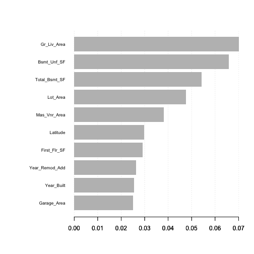
改使用’Cover’當作變數重要衡量法的結果與上面差很多。
|
1 2 |
# variable importance plot using 'cover' xgb.plot.importance(importance_matrix, top_n = 10, measure = "Cover") |
Partial dependence plots
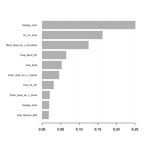
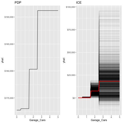
PDPs和ICE的運作與之前gbm套件是相似的。唯一差別在於你必須在partial()函數中加入訓練資料(train = features_train)(因為在此case中,partial無法自動擷取object所使用的training data)。我們以Garage_Cars為範例。
|
1 2 3 4 5 6 7 8 9 10 11 |
pdp % partial(pred.var = "Garage_Cars", n.trees = 1576, grid.resolution = 100, train = features_train) %>% autoplot(rug = TRUE, train = features_train) + scale_y_continuous(labels = scales::dollar) + ggtitle("PDP") ice % partial(pred.var = "Garage_Cars", n.trees = 1576, grid.resolution = 100, train = features_train, ice = TRUE) %>% autoplot(rug = TRUE, train = features_train, alpha = .1, center = TRUE) + scale_y_continuous(labels = scales::dollar) + ggtitle("ICE") |
|
1 |
gridExtra::grid.arrange(pdp, ice, nrow = 1) |
LIME
LIME內建提供給xgboost物件的功能(可以使用?model.type)。然而需要注意的是,要分析的局部觀察值需要採用與train, test相同的編碼處理程序(one-hot encoded)。並且當將資料投入lime::lime函式時,必須將其從matrix轉換成dataframe。
|
1 2 3 4 5 6 7 |
# one-hot encode the local observations to be assessed. local_obs_onehot # apply LIME explainer explanation plot_features(explanation) |
Predicting
最後,我們使用predict()函數來對新資料集進行預測。然而,不像gbm,我們並不需要提供樹模型的個數。
由下的結果可知,我們測試資料集的RMSE與先前gbm模型的RMSE(22K)是較低的(只差了$600左右,差距很小)。
|
1 2 3 4 5 |
# predict values for test data pred # results caret::RMSE(pred, response_test) |
|
1 2 |
## [1] 21433.41 |
h2o
R的h2O套件是一個強大高效能的java-based介面,允許基於local和cluster-based的佈署。該套件有相當完整的線上資源,包括方法、code文件與教學。
h2o的幾個特色包括:
- 在單一節點或多節點群集上進行分散式或平行式運算。
- 根據用戶指定的指標和使用者指定的相對容忍度收斂時,自動提前停止。
- 隨機GBM同時對欄位跟資料列進行抽樣(每次分割與每棵樹)以利得到廣義的解。
- 除了二項式binomial(Bernoulli)、高斯和多項式分佈函式外,亦支援指數型系列(Poisson, Gamma, Tweedie)和損失函數。
- Grid Search超參數優化和模型挑選。
- 數據分散(data-distributed) – 代表整個資料集不必侷限在單一節點的記憶體,能夠擴展到任意大小的訓練資料集。
- 使用直方圖(histogram)來近似連續變數來加速。
- 使用動態分箱法(dynamic binning),分箱的標準會依照每一顆樹模型切割時的最大最小值來動態調整。
- 使用平方誤差(squared error)來決定最適的切割點。
- factor levels沒有限制。
基本的h2o實作
|
1 2 |
h2o.no_progress() h2o.init(max_mem_size = "5g") |
|
1 2 3 4 5 6 7 8 9 10 11 12 13 14 15 16 17 18 19 20 21 |
## Connection successful! ## ## R is connected to the H2O cluster: ## H2O cluster uptime: 1 days 10 hours ## H2O cluster timezone: Asia/Taipei ## H2O data parsing timezone: UTC ## H2O cluster version: 3.22.1.1 ## H2O cluster version age: 3 months and 12 days !!! ## H2O cluster name: H2O_started_from_R_peihsuan_hxs725 ## H2O cluster total nodes: 1 ## H2O cluster total memory: 2.54 GB ## H2O cluster total cores: 4 ## H2O cluster allowed cores: 4 ## H2O cluster healthy: TRUE ## H2O Connection ip: localhost ## H2O Connection port: 54321 ## H2O Connection proxy: NA ## H2O Internal Security: FALSE ## H2O API Extensions: XGBoost, Algos, AutoML, Core V3, Core V4 ## R Version: R version 3.5.2 (2018-12-20) |
gbm.h2o函數可允許我們透過H2O套件來執行GBM。然而,在我們開始執行初始模型時,我們需要將訓練資料轉換成h2o物件。h2o.gbm預設會採用以下參數來建立GBM模型:
- number of tree (ntrees): 50
- learning rate (learning_rate): 0.1
- tree depth(max_depth): 5
- 末梢節點的最小觀測值個數 (min_rows): 10
- 對資料列和資料欄位沒有抽樣
|
1 2 3 4 5 6 7 8 9 10 11 12 13 14 15 16 17 |
# create feature names y x # turn training set into h2o object train.h2o # training basic GBM model with defaults h2o.fit1 x = x, y = y, training_frame = train.h2o, nfolds = 5 ) # assess model results h2o.fit1 |
|
1 2 3 4 5 6 7 8 9 10 11 12 13 14 15 16 17 18 19 20 21 22 23 24 25 26 27 28 29 30 31 32 33 34 35 36 37 38 39 40 41 42 |
## Model Details: ## ============== ## ## H2ORegressionModel: gbm ## Model ID: GBM_model_R_1554713367949_3 ## Model Summary: ## number_of_trees number_of_internal_trees model_size_in_bytes min_depth max_depth mean_depth min_leaves max_leaves mean_leaves ## 1 50 50 17160 5 5 5.00000 10 31 22.60000 ## ## ## H2ORegressionMetrics: gbm ## ** Reported on training data. ** ## ## MSE: 165078993 ## RMSE: 12848.31 ## MAE: 9243.007 ## RMSLE: 0.08504509 ## Mean Residual Deviance : 165078993 ## ## ## ## H2ORegressionMetrics: gbm ## ** Reported on cross-validation data. ** ## ** 5-fold cross-validation on training data (Metrics computed for combined holdout predictions) ** ## ## MSE: 707783149 ## RMSE: 26604.19 ## MAE: 15570.2 ## RMSLE: 0.1404869 ## Mean Residual Deviance : 707783149 ## ## ## Cross-Validation Metrics Summary: ## mean sd cv_1_valid cv_2_valid cv_3_valid cv_4_valid cv_5_valid ## mae 15547.765 721.0162 16325.277 16366.696 13728.291 15117.01 16201.549 ## mean_residual_deviance 7.0412026E8 1.68594576E8 6.8916365E8 1.12267443E9 3.96582368E8 5.8667603E8 7.2550477E8 ## mse 7.0412026E8 1.68594576E8 6.8916365E8 1.12267443E9 3.96582368E8 5.8667603E8 7.2550477E8 ## r2 0.8918067 0.02474849 0.8868936 0.8282497 0.92912257 0.91696167 0.89780617 ## residual_deviance 7.0412026E8 1.68594576E8 6.8916365E8 1.12267443E9 3.96582368E8 5.8667603E8 7.2550477E8 ## rmse 26165.846 3119.9976 26251.926 33506.336 19914.377 24221.396 26935.195 ## rmsle 0.13949537 0.010692091 0.13955544 0.16392557 0.14536715 0.11926634 0.12936236 |
跟XGBoost類似,我們可以使用自動停止功能,這樣就可以提高樹模型的個數,直到模型改善幅度減少或停止在終止訓練程序。亦可設定當執行時間超過一定水準後停止程序(參考max_runtime_secs)。
舉例來說,我們使用5000棵樹訓練一個預設參數的模型,但是設定當連續十棵樹模型在交叉驗證誤差上沒有進步就停止的指令。而在此例可以看到,模型在約使用3743棵樹模型後停止訓練過程,對應的交叉驗證誤差RMSE為$24,684。
|
1 2 3 4 5 6 7 8 9 10 11 12 13 14 |
# training basic GBM model with defaults h2o.fit2 x = x, y = y, training_frame = train.h2o, nfolds = 5, ntrees = 5000, stopping_rounds = 10, stopping_tolerance = 0, seed = 123 ) # model stopped after xx trees h2o.fit2@parameters$ntrees |
|
1 2 |
## [1] 3712 |
|
1 2 |
# cross validated RMSE h2o.rmse(h2o.fit2, xval = TRUE) |
|
1 2 |
## [1] 24683.95 |
Tuning
H2O套件提供需多可調整的參數。這部分值得你花時間閱讀相關的文件H2O.ai。在本筆記中,只會先專注在幾個較長使用的超參數組合。包括:
- 樹的複雜度
- ntrees: 使用樹模型個數
- max_depth: 每棵樹的深度
- min_rows: 末梢節點中所允許的最少觀測值個數
- 學習步伐
- learn_rate: 損失函數梯度下降的步伐
- learn_rate_annealing: 允許使用高的學習步伐當作初始值,但隨著樹個數的增加而降低。
- 加入隨機的特性
- sample_rate: 建置每棵數所抽樣的訓練資料列數。
- col_sample_rate: 建置每棵樹所抽樣的欄位數(跟xgboost套件中的colsample_bytree是一樣的)。
值得注意的是,還有能夠控制類別變數和連續變數如何編碼、分箱、切割的參數。預設的參數可以得到相當不錯的結果,但在特定情境中仍能透過調整這些小地方來微提高模型的效果。
執行h2o模型的grid search tuning有兩種選擇:full 或 random discrete grid search。
Full grid search
在full cartesian grid search法中,會完整依序執行grid中指定的所有超參數組合。這就是我們先前在gbm和xgboost手動撰寫for迴圈執行的參數校正過程。然而為了加快H2O訓練的過程,可以使用驗證資料集(validation set)來取代k-fold cross validation。
以下我們製造一個參數的grid,包含468(=3*3*3*2*3*3)種超參數排列組合。我們使用h2o.grid()來執行full grid search並同時設定停止參數來節省訓練的時間。
|
1 2 3 4 5 6 7 8 9 10 11 12 13 14 15 16 17 18 19 20 21 22 23 24 25 26 27 28 29 30 31 |
# create training & validation sets split train valid # create hyperparameter grid hyper_grid max_depth = c(1, 3, 5), min_rows = c(1, 5, 10), learn_rate = c(0.01, 0.05, 0.1), learn_rate_annealing = c(.99, 1), sample_rate = c(.5, .75, 1), col_sample_rate = c(.8, .9, 1) ) # perform grid search system.time( grid algorithm = "gbm", grid_id = "gbm_grid1", x = x, y = y, training_frame = train, validation_frame = valid, hyper_params = hyper_grid, ntrees = 5000, stopping_rounds = 10, stopping_tolerance = 0, seed = 123 ) ) |
full grid search所花的時間約為31分鐘。
|
1 2 3 4 5 6 7 |
# collect the results and sort by our model performance metric of choice grid_perf grid_id = "gbm_grid1", sort_by = "mse", decreasing = FALSE ) grid_perf |
|
1 2 3 4 5 6 7 8 9 10 11 12 13 14 15 16 17 18 19 20 21 22 23 24 25 26 27 28 29 30 |
## H2O Grid Details ## ================ ## ## Grid ID: gbm_grid1 ## Used hyper parameters: ## - col_sample_rate ## - learn_rate ## - learn_rate_annealing ## - max_depth ## - min_rows ## - sample_rate ## Number of models: 486 ## Number of failed models: 0 ## ## Hyper-Parameter Search Summary: ordered by increasing mse ## col_sample_rate learn_rate learn_rate_annealing max_depth min_rows sample_rate model_ids mse ## 1 1.0 0.05 1.0 5 1.0 0.75 gbm_grid1_model_213 4.64582634567234E8 ## 2 0.8 0.01 1.0 5 1.0 0.5 gbm_grid1_model_46 4.748883474543088E8 ## 3 0.8 0.01 1.0 5 1.0 0.75 gbm_grid1_model_208 4.7571620498865277E8 ## 4 0.9 0.01 1.0 5 1.0 0.75 gbm_grid1_model_209 4.775898758772956E8 ## 5 1.0 0.01 1.0 5 1.0 0.5 gbm_grid1_model_48 4.7783819706988806E8 ## ## --- ## col_sample_rate learn_rate learn_rate_annealing max_depth min_rows sample_rate model_ids mse ## 481 1.0 0.01 0.99 1 5.0 1.0 gbm_grid1_model_381 2.9511012504833984E9 ## 482 1.0 0.01 0.99 1 1.0 1.0 gbm_grid1_model_327 2.9511012504833984E9 ## 483 1.0 0.01 0.99 1 10.0 1.0 gbm_grid1_model_435 2.9511012504833984E9 ## 484 1.0 0.01 0.99 1 1.0 0.75 gbm_grid1_model_165 2.951772702040925E9 ## 485 1.0 0.01 0.99 1 5.0 0.75 gbm_grid1_model_219 2.951772702040925E9 ## 486 1.0 0.01 0.99 1 10.0 0.75 gbm_grid1_model_273 2.951772702040925E9 |
由以上資訊可知,模型切割數超過1次的深度、慢的學習步伐和隨機觀測值抽樣是表現的最不錯的組合類型。
我們亦可查看更多有關最佳模型的詳細資訊。最佳模型可達到的驗證誤差RMSE為$21,554。
|
1 2 3 4 5 6 |
# Grab the model_id for the top model, chosen by validation error best_model_id best_model # Now let’s get performance metrics on the best model h2o.performance(model = best_model, valid = TRUE) |
|
1 2 3 4 5 6 7 8 9 |
## H2ORegressionMetrics: gbm ## ** Reported on validation data. ** ## ## MSE: 464582635 ## RMSE: 21554.18 ## MAE: 14389.8 ## RMSLE: 0.1268479 ## Mean Residual Deviance : 464582635 |
Random discrete grid search
當想要測試的超參數排列組合非常多時,每增加一個參數都對grid search所需完成的時間有巨大的影響。因此,h2o亦有提供Random discrete的grid search path法,採取隨機挑選超參數組合來執行,直到指定程度的改善幅度被達成或超過一定的執行時間或只執行過一定的模型數量時(或以上條件的組合)則停止。雖然說Random discrete path不一定會找到最適的模型,但在一定程度上可以找到相當不錯的模型。
以下便採用Random Discrete Path法來執行和剛剛一模一樣的hyperparameter grid。不過,在此我們會加入新的search條件:當連續有10個模型效果都無法超越目前最佳的模型獲得0.5%的MSE改善時,則停止。如果持續有在獲得改善,但超過360秒(60分鐘)時,也停止程序。
|
1 2 3 4 5 6 7 8 9 10 11 12 13 14 15 16 17 18 19 20 21 22 23 24 25 26 |
# random grid search criteria search_criteria strategy = "RandomDiscrete", stopping_metric = "mse", stopping_tolerance = 0.005, stopping_rounds = 10, max_runtime_secs = 60*60 ) # perform grid search system.time( grid algorithm = "gbm", grid_id = "gbm_grid2", x = x, y = y, training_frame = train, validation_frame = valid, hyper_params = hyper_grid, search_criteria = search_criteria, # add search criteria ntrees = 5000, stopping_rounds = 10, stopping_tolerance = 0, seed = 123 ) ) |
|
1 2 3 |
## user system elapsed ## 38.949 11.738 3602.198 |
在此例子中,Random Grid Search花了約60分鐘(=3600/60),評估了154/486個模型(32%)。
|
1 2 3 4 5 6 7 |
# collect the results and sort by our model performance metric of choice grid_perf grid_id = "gbm_grid2", sort_by = "mse", decreasing = FALSE ) grid_perf |
|
1 2 3 4 5 6 7 8 9 10 11 12 13 14 15 16 17 18 19 20 21 22 23 24 25 26 27 28 29 30 31 |
## H2O Grid Details ## ================ ## ## Grid ID: gbm_grid2 ## Used hyper parameters: ## - col_sample_rate ## - learn_rate ## - learn_rate_annealing ## - max_depth ## - min_rows ## - sample_rate ## Number of models: 154 ## Number of failed models: 0 ## ## Hyper-Parameter Search Summary: ordered by increasing mse ## col_sample_rate learn_rate learn_rate_annealing max_depth min_rows sample_rate model_ids mse ## 1 0.9 0.01 1.0 3 1.0 0.75 gbm_grid2_model_45 4.748951758832882E8 ## 2 1.0 0.01 1.0 3 1.0 0.5 gbm_grid2_model_80 4.803434026601322E8 ## 3 1.0 0.1 1.0 3 1.0 0.75 gbm_grid2_model_17 4.926287246284121E8 ## 4 0.9 0.01 1.0 3 1.0 0.5 gbm_grid2_model_115 5.0211786533732516E8 ## 5 0.9 0.05 1.0 5 1.0 0.5 gbm_grid2_model_107 5.069315439854374E8 ## ## --- ## col_sample_rate learn_rate learn_rate_annealing max_depth min_rows sample_rate model_ids mse ## 149 1.0 0.01 0.99 1 10.0 0.75 gbm_grid2_model_146 3.4271307547685847E9 ## 150 1.0 0.01 0.99 1 5.0 0.75 gbm_grid2_model_24 3.4271307547685847E9 ## 151 0.8 0.01 0.99 1 10.0 0.75 gbm_grid2_model_41 3.427939673958527E9 ## 152 0.8 0.01 0.99 1 10.0 1.0 gbm_grid2_model_27 3.4288680514316573E9 ## 153 1.0 0.01 0.99 1 5.0 1.0 gbm_grid2_model_131 3.4293746592550063E9 ## 154 1.0 0.01 1.0 3 1.0 0.75 gbm_grid2_model_154 5.038339642534549E9 |
透過Random Grid Search所得到的最佳模型的交叉驗證RMSE為$21,792。雖然沒有full grid search找到的好($21,554),但通常兩者所找到模型的效果已是差不多的。
|
1 2 3 4 5 6 |
# Grab the model_id for the top model, chosen by validation error best_model_id best_model # Now let’s get performance metrics on the best model h2o.performance(model = best_model, valid = TRUE) |
|
1 2 3 4 5 6 7 8 9 |
## H2ORegressionMetrics: gbm ## ** Reported on validation data. ** ## ## MSE: 474895176 ## RMSE: 21792.09 ## MAE: 13738.25 ## RMSLE: 0.1245287 ## Mean Residual Deviance : 474895176 |
一旦我們找到了最佳模型後,就可以用所有的訓練資料再重新訓練一個模型。我們使用從full grid search所得到的最佳模型的參數組合並使用5-fold cross validation來估計穩健的誤差。
|
1 2 3 4 5 6 7 8 9 10 11 12 13 14 15 16 17 |
# train final model h2o.final x = x, y = y, training_frame = train.h2o, nfolds = 5, ntrees = 10000, learn_rate = 0.01, learn_rate_annealing = 1, max_depth = 3, min_rows = 10, sample_rate = 0.75, col_sample_rate = 1, stopping_rounds = 10, stopping_tolerance = 0, seed = 123 ) |
|
1 2 |
# model stopped after xx trees h2o.final@parameters$ntrees |
|
1 2 |
## [1] 8660 |
|
1 2 |
# cross validated RMSE h2o.rmse(h2o.final, xval = TRUE) |
|
1 2 |
## [1] 23214.71 |
Visualization
Variable importance
h2o套件有提供內建的變數重要性繪圖功能。該函式只有一個衡量變數重要性的方法-relative importance,一種衡量每一個變數在每一個模型中,平均能對loss function造成多少影響。能對損失函數帶來最大平均影響者的變數被當作最重要的變數,且其他變數的重要性也是相對於最重要變數所計算而得的數值。另外,vip套件亦可繪製h2o物件的變數重要性圖。
|
1 |
h2o.varimp_plot(h2o.final, num_of_features = 10) |
Partial dependence plots
我們亦可像之前一樣使用vip套件繪製PDP和ICE圖型來了解不同解釋變數邊際變動下對目標變數造成的影響。我們只需要透過一段專用函數,將投入的資料(newdata)轉換成h2o物件(as.h2o),並將預測的結果在轉換為data frame型態,在當成pred.fun的參數投入。
|
1 2 3 4 5 6 7 8 9 10 11 12 13 14 |
pfun as.data.frame(predict(object, newdata = as.h2o(newdata)))[[1L]] } pdp % partial( pred.var = "Gr_Liv_Area", pred.fun = pfun, # 研究一下 grid.resolution = 20, train = ames_train ) %>% autoplot(rug = TRUE, train = ames_train, alpha = .1) + scale_y_continuous(labels = scales::dollar) + ggtitle("PDP") |
|
1 2 3 4 5 6 7 8 9 10 11 |
ice % partial( pred.var = "Gr_Liv_Area", pred.fun = pfun, grid.resolution = 20, train = ames_train, ice = TRUE ) %>% autoplot(rug = TRUE, train = ames_train, alpha = .1, center = TRUE) + scale_y_continuous(labels = scales::dollar) + ggtitle("ICE") |
|
1 |
gridExtra::grid.arrange(pdp, ice, nrow = 1) |
h2o並沒有提供內建的ICE曲線繪圖功能,但是他可以繪製平均邊際效益(標準的PDP圖)外加衡量不確定性的一個標準誤差的PDP圖。
|
1 |
h2o.partialPlot(h2o.final, data = train.h2o, cols = "Overall_Qual") |
|
1 2 3 4 5 6 7 8 9 10 11 12 13 |
## PartialDependence: Partial Dependence Plot of model GBM_model_R_1554713367949_5 on column 'Overall_Qual' ## Overall_Qual mean_response stddev_response std_error_mean_response ## 1 Above_Average 173439.744454 59206.888258 1307.342580 ## 2 Average 169032.396430 58675.968674 1295.619387 ## 3 Below_Average 165991.718878 61198.281190 1351.314368 ## 4 Excellent 227862.381764 66306.055141 1464.098718 ## 5 Fair 161119.245285 62126.019654 1371.799687 ## 6 Good 185468.115459 62195.668588 1373.337600 ## 7 Poor 156505.758628 63260.388765 1396.847601 ## 8 Very_Excellent 228227.228142 66731.640843 1473.496042 ## 9 Very_Good 206801.916781 64639.301392 1427.295261 ## 10 Very_Poor 151217.679576 64366.405585 1421.269471 |
但不幸的事,h2o的函數會把類別變數的levels以字母排序的方式繪出,而pdp()函式則是以他們所指定的level順序繪出,使推理更加直觀。
|
1 2 3 4 5 6 7 8 9 10 11 12 13 14 15 16 17 18 19 20 21 22 23 24 |
pdp % partial( pred.var = "Overall_Qual", pred.fun = pfun, grid.resolution = 20, train = as.data.frame(ames_train) ) %>% autoplot(rug = TRUE, train = ames_train, alpha = .1) + scale_y_continuous(labels = scales::dollar) + ggtitle("PDP") ice % partial( pred.var = "Overall_Qual", pred.fun = pfun, grid.resolution = 20, train = as.data.frame(ames_train), ice = TRUE ) %>% autoplot(rug = TRUE, train = ames_train, alpha = .1, center = TRUE) + scale_y_continuous(labels = scales::dollar) + ggtitle("ICE") gridExtra::grid.arrange(pdp, ice, nrow = 1) |
LIME
LIME套件亦有提供內建的函數來處理h2o物件。
|
1 2 3 4 |
# apply LIME explainer explanation plot_features(explanation) |
Predicting
最後,我們可以使用h2o.predict()或predict()兩種方式來進行模型對新資料的預測,並使用h2o.performance()來衡量模型模型套用在測試資料集的成效。驗證結果的RMSE為$20,198,跟gbm和xgboost是類似的($21~22K)。
|
1 2 3 4 5 |
# convert test set to h2o object test.h2o # evaluate performance on new data h2o.performance(model = h2o.final, newdata = test.h2o) |
|
1 2 3 4 5 6 7 8 |
## H2ORegressionMetrics: gbm ## ## MSE: 407897003 ## RMSE: 20196.46 ## MAE: 12679.15 ## RMSLE: 0.1008391 ## Mean Residual Deviance : 407897003 |
|
1 2 |
# predict with h2o.predict h2o.predict(h2o.final, newdata = test.h2o) |
|
1 2 3 4 5 6 7 8 9 10 |
## predict ## 1 129814.6 ## 2 161987.0 ## 3 262990.7 ## 4 484455.6 ## 5 218094.0 ## 6 209430.8 ## ## [879 rows x 1 column] |
|
1 2 |
# predict values with predict predict(h2o.final, test.h2o) |
|
1 2 3 4 5 6 7 8 9 10 |
## predict ## 1 129814.6 ## 2 161987.0 ## 3 262990.7 ## 4 484455.6 ## 5 218094.0 ## 6 209430.8 ## ## [879 rows x 1 column] |
小結
- Gradient Boosting Machines (GBM)是一個強大的集成學習演算法,通常具有一流的預測能力。雖然相較於其他演算法它比較不直覺且需要大型運算,但絕對是機器學習工具箱的必備款!
參考連結:
- Gradient Boosting Machines (GBM)
- 類別資料的處理(有序、無序):one-hot encoding
- Choosing the right Encoding method-Label vs OneHot Encoder
更多Decision Tree相關的統計學習筆記:
Random Forests 隨機森林 | randomForest, ranger, h2o | R語言
Decision Tree 決策樹 | CART, Conditional Inference Tree, RandomForest
Regression Tree | 迴歸樹, Bagging, Bootstrap Aggregation | R語言
Tree Surrogate | Tree Surrogate Variables in CART | R 統計
更多Regression相關統計學習筆記:
Linear Regression | 線性迴歸模型 | using AirQuality Dataset
Logistic Regression 羅吉斯迴歸 | part1 – 資料探勘與處理 | 統計 R語言
Logistic Regression 羅吉斯迴歸 | part2 – 模型建置、診斷與比較 | R語言
Regularized Regression | 正規化迴歸 – Ridge, Lasso, Elastic Net | R語言
更多Clustering集群分析統計學習筆記:
Partitional Clustering 切割式分群 | Kmeans, Kmedoid | Clustering 資料分群
Hierarchical Clustering 階層式分群 | Clustering 資料分群 | R 統計
其他統計學習筆記: