


Hierarchical Clustering, 屬於資料分群的一種方法。資料分群屬於非監督式學習,處理的資料是沒有正確答案/標籤/目標變數可參考的。常見的分群方法包括著名的kmeans, hierarchical clustering,分別使用不同分群演算邏輯。本篇將介紹階層式分群的實作與特色。
資料分群簡介
- 資料分群是一個將資料分割成數個子集合的方法,主要目的包括:
- 找出資料中相近的群聚(clusters),
- 找出各群的代表點。代表點可以是群聚中的中心點(centroids)或是原型(prototypes)。
- 透過各群的代表點,可以達到幾個目標:
- 資料壓縮
- 降低雜訊
- 降低計算量
- 資料分群將依據資料自身屬性計算彼此間的相似度(物以類聚),而「相似度」主要有兩種型態:
- 「Compactness」:目標是讓子集合間差異最大化,子集合內差異最小化。如階層式分群和K-means分群。
- 「Connectedness」:目標是將可串連在一起的個體分成一群。如譜分群(Spectral Clustering)。
- 資料分群屬於非監督式學習法(Unsupervised Learning),即資料沒有標籤(unlabeled data)或沒有標準答案,無法透過所謂的目標變數(response variable)來做分類之訓練。也因為資料沒有標籤之緣故,與監督式學習法和強化式學習法不同,非監督式學習法無法衡量演算法的正確率。
資料分群系列文章會依序介紹以下幾種常見的分群方法:
- 階層式分群(hierarchical clustering)
- 聚合式階層分群法 Agglomerative Hierarchical Clustering
- 分裂式階層分群法 Divisive Hierarchical Clustering
- 最佳分群群數(Determining Optimal Clusters)
- 切割式分群(partitional clustering)
- K-means
- K-medoid
- 最佳分群群數(Determining Optimal Clusters)
- 譜分群(Spectral Clustering)
1. 階層式分群(Hierarchical clustering)
- 階層分群法的概念是在分群中建立分群,並不需要預先設定分群數。
- 產生的分群結果為一目瞭然的樹狀結構圖(又稱作dendrogram)。
- 群數(number of clusters)可由大變小(divisive hierarchical clustering),或是由小變大(agglomerative hierarchical clustering),透過群聚反覆的分裂和合併後,在選取最佳的群聚數。
- 階層式分群兩種演算法:
- 當採行聚合法,又稱作AGNES(Agglomerative Nesting),資料會由樹狀結構的底部開始開始逐次合併 (bottom-up),在R語言中所使用的函數為hclust()[in stat package]或agnes[in cluster package],擅於處理與識別小規模群聚
- 當採行分裂法,又稱作DIANA(Divisive Analysis),資料則會由樹狀結構的頂部開始逐次分裂(top-down),在R語言中使用的套件為diana()[in cluster package],擅於處理與識別大規模群聚。
- 階層分群可被用運用數值與類別資料。
1-1. 聚合式階層群聚法(AGNES, bottom-up)
我們使用Iris資料集-經典的鳶尾花資料來進行聚合式階層群聚法之說明。(*注意,資料必須先預處理遺失值的部分,比如說使用na.omit(data)。)
|
1 2 3 4 5 6 7 8 9 |
head(iris) # Sepal.Length Sepal.Width Petal.Length Petal.Width Species # 1 5.1 3.5 1.4 0.2 setosa # 2 4.9 3.0 1.4 0.2 setosa # 3 4.7 3.2 1.3 0.2 setosa # 4 4.6 3.1 1.5 0.2 setosa # 5 5.0 3.6 1.4 0.2 setosa # 6 5.4 3.9 1.7 0.4 setosa |
因為分群法為非監督式學習法,專處理無標籤(un-labeled)或無標準答案的資料分群,故我們將分類結果欄位Species從我們的inputData刪除。
|
1 2 3 4 5 6 7 8 9 10 |
inputData head(inputData) # Sepal.Length Sepal.Width Petal.Length Petal.Width # 1 5.1 3.5 1.4 0.2 # 2 4.9 3.0 1.4 0.2 # 3 4.7 3.2 1.3 0.2 # 4 4.6 3.1 1.5 0.2 # 5 5.0 3.6 1.4 0.2 # 6 5.4 3.9 1.7 0.4 |
在進行聚合式群聚法前,我們先簡單介紹幾個hclust()函數中的重要參數:
- d : 由dist()函數計算出來資料兩兩間的相異度矩陣(dissimilarity matrix),即兩兩資料間的距離矩陣。
- method: 群(clusters)聚合或連結的方式。包括:single(單一)、complete(完整)、average(平均)、Ward’s(華德)和 centroid(中心)等法。其中又以average(平均)聚合方法被認為是最適合的。不同方法對階層分群結果亦有極大影響。
R語言hclust()套件中提供群聚距離演算法來衡量兩群聚的不相似度,最常見的幾種演算法如下:
- 單一連結聚合演算法(single-linkage agglomerative algorithm): 群與群的距離定義為不同群聚中最近的兩個點的距離。傾向產生較於緊緻(compact)的群聚。
$$d(C_{i},C_{j})=\min_{a\in C_{i},b\in C_{j}}d(a,b)$$ - 完整連結聚合演算法(complete-linkage agglomerative algorithm): 群與群的距離定義為不同群聚中最遠的兩個點的距離。傾向產生較於長(long)、鬆散(loose)的群聚。
$$d(C_{i},C_{j})=\max_{a\in C_{i},b\in C_{j}}d(a,b)$$ - 平均連結聚合演算法(average-linkage agglomerative algorithm): 群與群的距離定義為不同群聚中各點與各點距離總和的平均。
$$d(C_{i},C_{j})=\sum_{a\in C_{i},b\in C_{j}}\frac{d(a,b)}{|C_{i}||C_{j}|}$$
其中,\(|C_{i}|\)和\(|C_{j}|\)分別為群聚\(C_{i}\)和\(C_{j}\)的大小。 - 中心連結聚合演算法(centroid-linkage agglomerative algorithm): 群與群的距離定義為不同群聚中心點之間的距離。
$$d(A,B)= d(\bar{X}_{A},\bar{X}_{B})=\|\bar{X}_{A}-\bar{X}_{B}\|^2$$ - 華德最小變異法(Ward’s Minimum Variance): 最小化各群聚內變異加總(minimize the total within-cluster variance)。主要用來尋找緊湊球型的群聚。反覆比較每對資料合併後的群內總變異數的增量,並找增量最小的組別優先合併。越早合併的子集表示其間的相似度越高。而使用華德最小變異法的前提為,初始各點資料距離必須是歐式距離的平方和(Squared Euclidean Distance)。在R套件hclust將參數設為method = “ward.D2″(不是”ward.D”)。(華德法參考文獻)
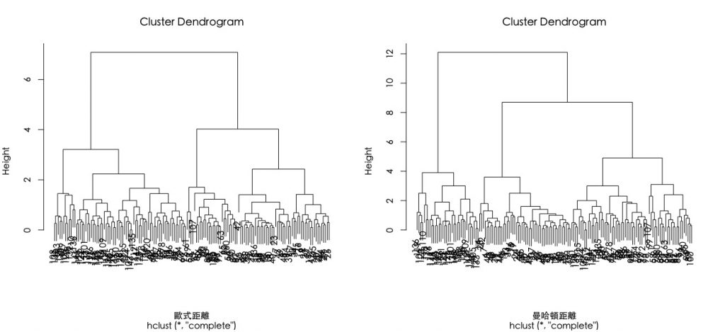
我們先來試試,不同的資料點間距離矩陣計算之效果。即調整dist()中參數method。
- 歐式距離(以二維空間為例):最常用也是最重要的距離計算法。
$$d(P_{1},P_{2})=\sqrt{(x_{1}-x_{2})^2+(y_{1}-y_{2})^2}$$ - 曼哈頓距離(以二維空間為例):
$$d(P_{1},P_{2})=|x_{1}-x_{2}|+|y_{1}-y_{2}|$$
|
1 2 3 4 5 6 7 8 9 10 11 12 13 14 15 16 17 18 |
# 由於階層式分群是依據個體間的「距離」來計算彼此的相似度。 # 我們會先使用dist()函數,來計算所有資料個體間的「距離矩陣(Distance Matrix)」 # 而「距離」的算法又有:(1)歐式距離(2)曼哈頓距離 E.dist M.dist # 讓圖形以一行兩欄的排版方式呈現,如要還原請用dev.off() par(mfrow=c(1,2)) # 將以上資料間距離作為參數投入階層式分群函數:hclust() # 使用歐式距離進行分群 h.E.cluster plot(h.E.cluster, xlab="歐式距離",family="黑體-繁 中黑") # 使用曼哈頓距離進行分群 h.M.cluster plot(h.M.cluster, xlab="曼哈頓距離", family="黑體-繁 中黑") |
可發現不同資料距離計算會有不同分群結果。
- Height表示n-1組實數值。各值為使用特定聚合方法計算出來的標準數值。
比較不同歐式距離搭配不同聚合演算法的分群結果。
|
1 2 3 4 5 6 7 |
dev.off() par(mfrow= c(3,2),family="黑體-繁 中黑") plot(hclust(E.dist, method="single"),xlab = "最近聚合法:single-linkage") # 最近法 plot(hclust(E.dist, method="complete"), xlab = "最遠聚合法:complete-linkage") # 最遠法 plot(hclust(E.dist, method="average"), xlab = "平均聚合法: average-linkage") # 平均法 plot(hclust(E.dist, method="centroid"), xlab = "中心法: centroid-linkage") # 中心法 plot(hclust(E.dist, method="ward.D2"), xlab = "華德法: Ward's Method") # 華德法 |
從下圖可以發現群聚數結構的幾個特徵:
- Single-linkage法具有「大者恆大」之效果。
- 而 complete linkage 和 average linkage 比較具有「齊頭並進」之效果。
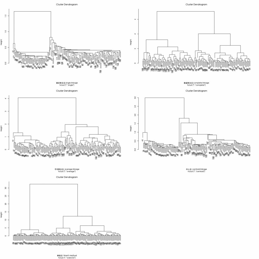
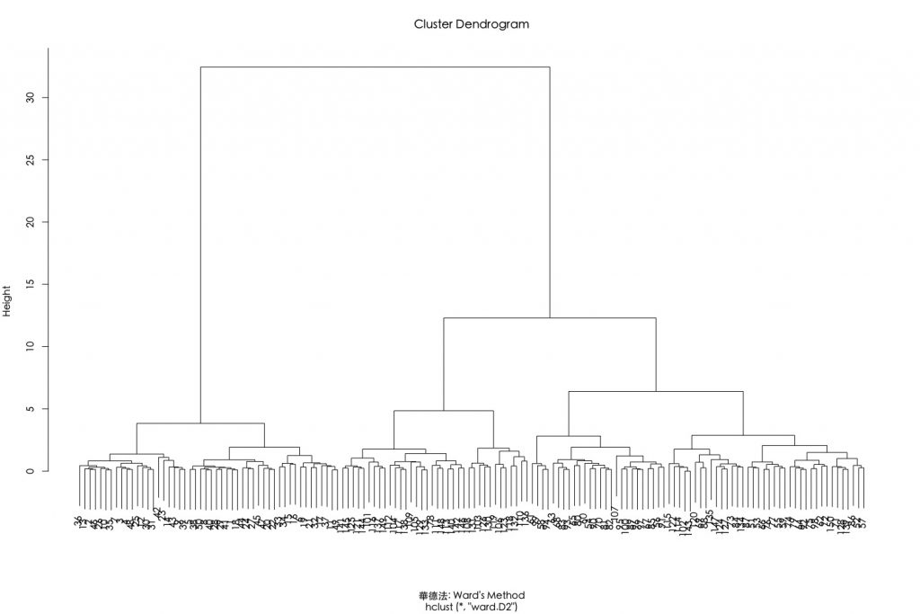
接著,我們聚焦在採用歐式距離搭配華德最小變異聚合演算法。可透過設定hclust()參數method=”ward.D2″。
|
1 2 3 |
dev.off() par(family="黑體-繁 中黑") plot(hclust(E.dist, method="ward.D2"), xlab = "華德法: Ward's Method") |
以上結果也可以使用anges()函數來執行。此函數跟hclust()很類似,不同之處是該函數能另外計算聚合係數(agglomerative coefficient)。聚合係數是衡量群聚結構被辨識的程度,聚合係數越接近1代表有堅固的群聚結構(strong clustering structure)。在這個使用歐式距離搭配華德連結演算法的群聚係數有高達99%的表現。
|
1 2 3 4 5 6 |
# Compute with agnes library(cluster) hc2 # Agglomerative coefficient hc2$ac ## [1] 0.9908772 |
我們可以用聚合係數來比較多組分群連結演算法的效果。此範例中又以華德法表現最好。
|
1 2 3 4 5 6 7 8 9 10 11 12 |
# methods to assess m names(m) # function to compute coefficient ac agnes(E.dist, method = x)$ac } map_dbl(m, ac) #Apply a function to each element of a vector # average single complete ward # 0.9300174 0.8493364 0.9574622 0.9908772 |
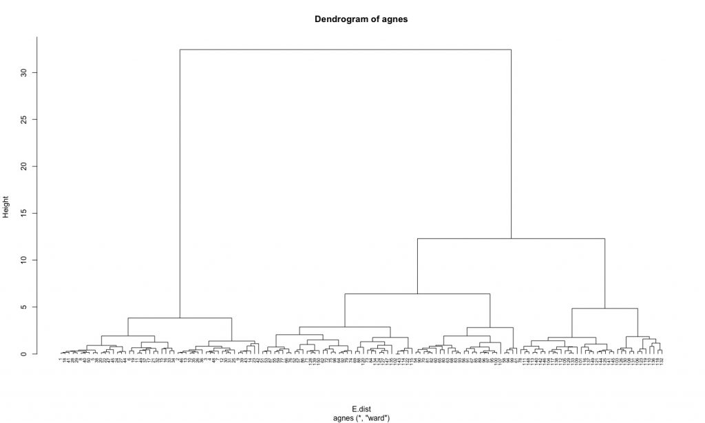
若遇將agnes()產生的樹狀圖繪出可使用函數pltree()。可以發現結果大致上與hclust()結果差不多。
|
1 2 3 |
dev.off() hc2 pltree(hc2, cex = 0.6, hang = -1, main = "Dendrogram of agnes") |
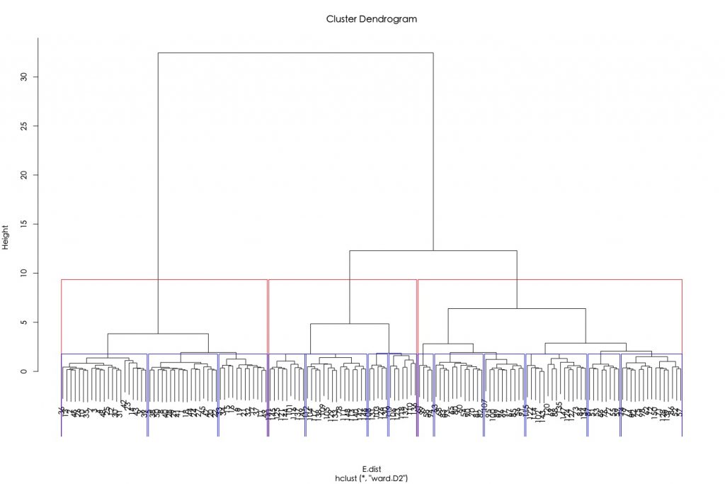
對階層分群結果產生的樹狀結構進行截枝可以將觀測值分成數群。截肢方法有兩種:
- 指定所要的分群數: rect.hclust(k=…)、cutree(k=…)
- 指定截枝的位置: rect.hclust(h=…)
比如說,指定將資料分成3群與13群。
|
1 2 3 4 |
h.E.Ward.cluster plot(h.E.Ward.cluster) rect.hclust(tree =h.E.Ward.cluster, k = 3, border = "red") rect.hclust(tree =h.E.Ward.cluster, k = 13, border = "blue") |
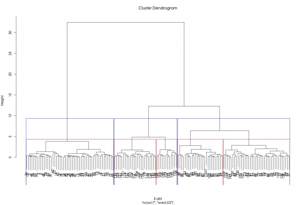
比如說,指定截枝高度分別為4和10,可分別將資料分成5組跟3組。
|
1 2 3 4 |
h.E.Ward.cluster plot(h.E.Ward.cluster) rect.hclust(tree =h.E.Ward.cluster, h = 4, border = "red") rect.hclust(tree =h.E.Ward.cluster, h = 10, border = "blue") |
如果要將資料標記上分群結果,可使用cutree(),並指定參數k為所欲截枝群樹。
|
1 2 3 4 5 6 7 |
h.E.Ward.cluster cut.h.cluster cut.h.cluster # [1] 1 1 1 1 1 1 1 1 1 1 1 1 1 1 1 1 1 1 1 1 1 1 1 1 1 1 1 1 1 1 1 1 1 1 1 1 1 1 1 1 1 1 1 1 1 1 1 1 1 1 2 2 2 2 2 # [56] 2 2 2 2 2 2 2 2 2 2 2 2 2 2 2 2 2 2 2 2 2 2 3 2 2 2 2 2 2 2 2 2 2 2 2 2 2 2 2 2 2 2 2 2 2 3 2 3 3 3 3 2 3 3 3 # [111] 3 3 3 2 2 3 3 3 3 2 3 2 3 2 3 3 2 2 3 3 3 3 3 2 2 3 3 3 2 3 3 3 2 3 3 3 2 3 3 2 |
分群結果和實際結果比較。
|
1 2 3 4 5 6 |
table(cut.h.cluster, iris$Species) # cut.h.cluster setosa versicolor virginica # 1 50 0 0 # 2 0 49 15 # 3 0 1 35 |
將資料分群的混淆矩陣視覺化。
|
1 |
plot(table(iris$Species, cut.h.cluster), main = "Confusion Matrix for Species Clustering", xlab = "Species", ylab = "Cluster") |
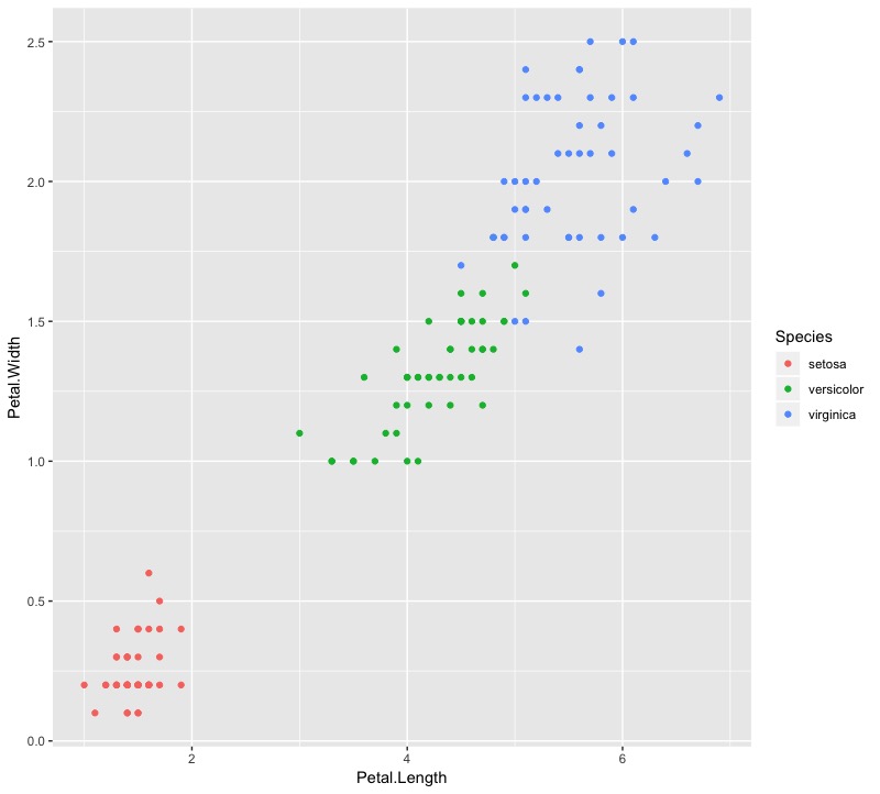
可以發現,屬於setosa種類的都被很好的分到第一群,屬於versicolor主要被分到第二群,但virginica似乎沒有分得很好。
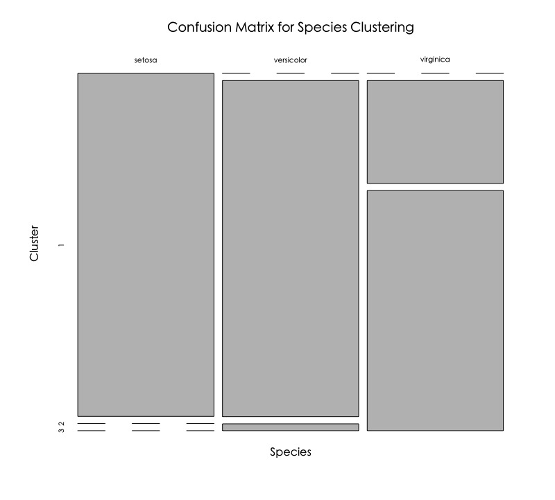
如果回頭看一下原始資料分佈長相,可以發現versicolor和virginica其實部分資料靠得很近,因此兩種Species被分到第二和第三群也是合理的。
|
1 2 |
ggplot(data = iris,mapping = aes(x = Petal.Length, y = Petal.Width)) + geom_point(aes(col = Species)) |
1-2. 分裂式階層群聚法(DIANA, top-down)
我們使用R內建的USArrests資料集來進行說明。進行分群前,我們先將資料預處理,包括遺失值忽略以及標準化(0~1)。
|
1 2 3 4 5 6 7 8 9 10 11 12 13 |
head(USArrests) # Murder Assault UrbanPop Rape # Alabama 13.2 236 58 21.2 # Alaska 10.0 263 48 44.5 # Arizona 8.1 294 80 31.0 # Arkansas 8.8 190 50 19.5 # California 9.0 276 91 40.6 # Colorado 7.9 204 78 38.7 inputData USArrests %>% na.omit() %>% scale() # scaling/standardizing the data |
diana()函數運作方式很類似agnes(),只差diana沒有method參數。
|
1 2 3 4 5 6 7 8 9 |
# compute divisive hierarchical clustering diana_clust # Divise coefficient; amount of clustering structure found diana_clust$dc ## [1] 0.8514345 # plot dendrogram pltree(diana_clust, cex = 0.6, hang = -1, main = "Dendrogram of diana") |
由分裂式階層分群演算法產出的樹狀圖結果如下:
- 葉節點(末梢節點)代表個別資料點。
- 垂直座標軸的Height代表群聚間的(不)相似度((dis)similarity), 群聚的高度(height)越高,代表觀測值間越不相似(組內變異越大)。需要注意的是,要總結兩個觀測值的相似度,只能用兩觀測值何時被第一次合併的群聚高度來做判斷,而不能以水平軸的距離來評估。
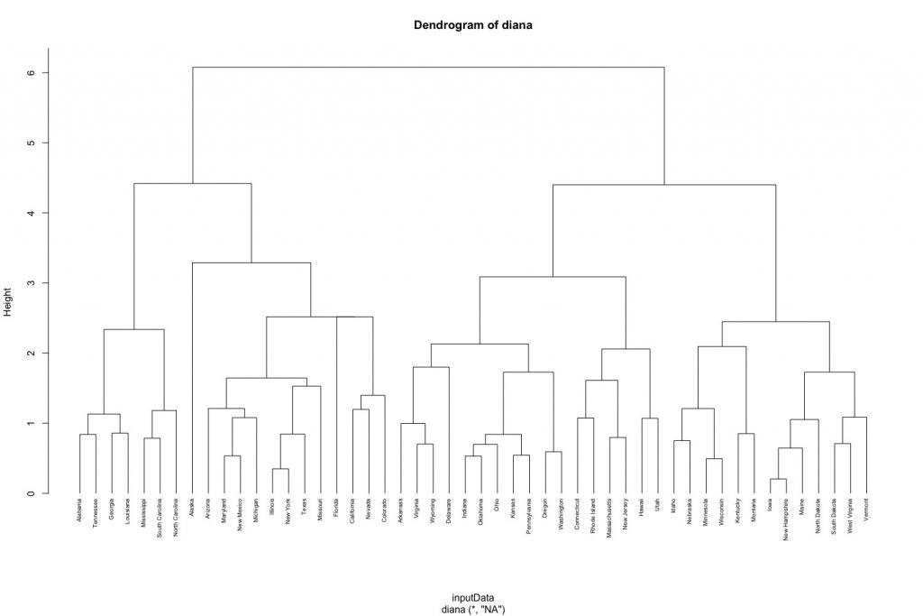
另外,我們可以透過縱軸的群聚高度來決定分群數目。我們可以使用cutree()函數來得到各觀測值被分類到的群。
|
1 2 3 4 5 |
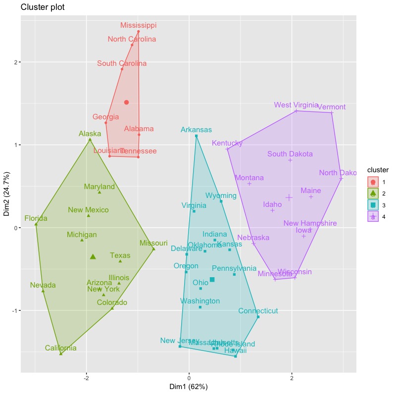
# Cut diana() tree into 4 groups diana_clust group group # [1] 1 2 2 3 2 2 3 3 2 1 3 4 2 3 4 3 4 1 4 2 3 2 4 1 2 4 4 2 4 3 2 2 1 4 3 3 3 3 3 1 4 1 2 3 4 3 3 4 4 3 |
我們使用factoextra套件中的fviz_clusterc函數來將分群結果視覺化。
|
1 2 |
library(factoextra) fviz_cluster(list(data = inputData, cluster = group)) |
1-3. 決定階層式分群最佳群聚數
1-3-1. Elbow Method
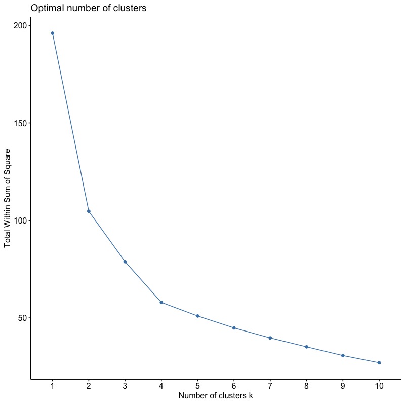
使用函數fviz_nbclust(),並將參數FUN指定為hcut(表階層式分群法)。wss代表組內平方誤差。
|
1 |
fviz_nbclust(inputData, FUN = hcut, method = "wss") |
由結果圖可知根據Elbow法,最佳分群數目為4群。
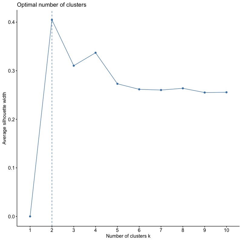
1-3-2. Average Silhouette Method
將method參數改為silhouette。
|
1 |
fviz_nbclust(x = inputData,FUNcluster = hcut, method = "silhouette") |
根據Average Silhouette Width,最佳分群數目為2 群。
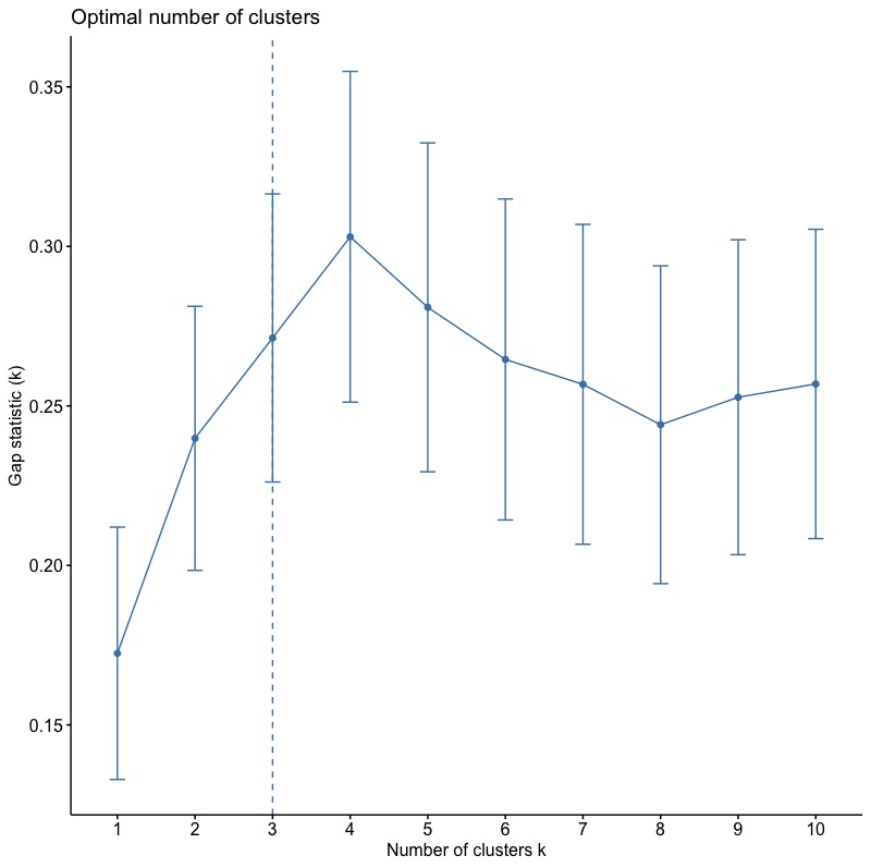
1-3-3. Gap Statistic Method
使用clusGap()函數。
|
1 2 |
gap_stat fviz_gap_stat(gap_stat) |
根據Gap(k)統計量,最佳分群數為3群。(*\(Gap(k)\geq Gap(k+1) – s_{k+1}\))
總結
- 階層分群主要受:資料個體兩兩間距離矩陣衡量方法與群與群連結方法所影響。
- 階層分群優點包括:
- 概念簡單且樹狀圖(dendrogram)結果一目瞭然。
- 只需要資料點間距離即可產出分群結果。
- 可以應用在數值或類別資料。
- 但缺點就是運算速度,以及不適用處理大量資料。運算速度方面,可以考慮其他R套件如fastcluster中的hclust函數,執行上會比一般hclust更有效率。
更多統計模型筆記連結:
- Linear Regression | 線性迴歸模型 | using AirQuality Dataset
- Regularized Regression | 正規化迴歸 – Ridge, Lasso, Elastic Net | R語言
- Logistic Regression 羅吉斯迴歸 | part1 – 資料探勘與處理 | 統計 R語言
- Logistic Regression 羅吉斯迴歸 | part2 – 模型建置、診斷與比較 | R語言
- Decision Tree 決策樹 | CART, Conditional Inference Tree, Random Forest
- Regression Tree | 迴歸樹, Bagging, Bootstrap Aggregation | R語言
- Random Forests 隨機森林 | randomForest, ranger, h2o | R語言
- Gradient Boosting Machines GBM | gbm, xgboost, h2o | R語言
- Hierarchical Clustering 階層式分群 | Clustering 資料分群 | R統計
- Partitional Clustering | 切割式分群 | Kmeans, Kmedoid | Clustering 資料分群
- Principal Components Analysis (PCA) | 主成份分析 | R 統計
參考: